Neoclassical growth model

The deterministic neoclassical (Ramsey–Cass–Koopmans) growth model is the gentlest introduction: one state variable, one value function, and a familiar calibration. For validation, the example creates a second parameter instance that satisfies a closed-form restriction. A representative household chooses consumption to solve

\[\max_{c} \int_0^\infty e^{-\rho t}\, \frac{c^{1-\gamma}}{1-\gamma}\, dt \qquad \text{subject to} \qquad \dot k = A k^\alpha - \delta k - c,\]

and the value function $v(k)$ solves the Hamilton–Jacobi–Bellman equation

\[\rho\, v(k) = \max_{c}\; \frac{c^{1-\gamma}}{1-\gamma} + v'(k)\,\bigl(A k^\alpha - \delta k - c\bigr),\]

with first-order condition $c = v'(k)^{-1/\gamma}$.

This is the same model solved step by step in Getting started. Here it is packaged the way the rest of the examples are — parameters in a struct, the equation as a callable on it — and the numerical solution is plotted against the closed-form benchmark.

Defining the model

The parameters live in a struct:

using EconPDEs, Plots, Printf

Base.@kwdef struct NeoclassicalGrowthModel
    A::Float64 = 0.5     # productivity
    α::Float64 = 0.3     # capital share
    δ::Float64 = 0.05    # depreciation
    ρ::Float64 = 0.05    # discount rate
    γ::Float64 = 2.0     # relative risk aversion
end

Main.NeoclassicalGrowthModel

The default parameters match the introductory calibration:

m = NeoclassicalGrowthModel()

Main.NeoclassicalGrowthModel(0.5, 0.3, 0.05, 0.05, 2.0)

To validate the full numerical solution, we also build a second instance that imposes a restriction with a closed-form solution:

\[\rho = \delta(\alpha \gamma - 1), \qquad \alpha\gamma > 1.\]

In that case the optimal policy and value function are

\[c(k) = \phi A k^\alpha, \qquad v(k) = \frac{(\phi A)^{-\gamma} k^{1-\alpha\gamma}}{1-\alpha\gamma}, \qquad \phi = 1 - \frac{1}{\gamma}.\]

The closed-form instance is used only as a validation benchmark.

γ_benchmark = 4.0
m_benchmark = NeoclassicalGrowthModel(;
    γ = γ_benchmark,
    ρ = m.δ * (m.α * γ_benchmark - 1),
)

Main.NeoclassicalGrowthModel(0.5, 0.3, 0.05, 0.009999999999999998, 4.0)

Defining the grid

We define the grid, a NamedTuple keyed by capital $k$. We center it on the benchmark steady state $\bar k$ (where $\alpha A \bar k^{\alpha-1} = \rho + \delta$), spanning $0.1\bar k$ to $5\bar k$.

(; A, α, δ, ρ, γ) = m_benchmark
φ = 1 - 1 / γ
k̄ = (α * A / (ρ + δ))^(1 / (1 - α))
stategrid = (; k = range(0.1 * k̄, 5 * k̄, length = 1000))

(k = 0.37024203699314673:0.01816001983249669:18.512101849657338,)

Defining an initial guess

We define the initial guess, a NamedTuple keyed by the unknown $v$ — one value per grid point, the generic value of consuming gross output forever. These names (and the finite differences of $v$, such as vk_up) are what reappear in the equation below.

guess = (; v = [(A * k^α)^(1 - γ) / (1 - γ) / ρ for k in stategrid[:k]])

(v = [-652.1260939495407, -624.6192482188261, -599.4521923356804, -576.3341604169608, -555.0209838169578, -535.3060790466031, -517.0134547055283, -499.9922277800587, -484.11228175498326, -469.2607979704295  …  -19.441276577622528, -19.423975582873183, -19.406707059392076, -19.389470914251966, -19.372267054882926, -19.355095389070556, -19.33795582495434, -19.320848271025916, -19.303772636127363, -19.286728829449533],)

We also define the closed-form policy and value functions, used later to validate the numerical solution:

closed_form_consumption(k) = φ * A * k^α
closed_form_value(k) = (φ * A)^(-γ) * k^(1 - α * γ) / (1 - α * γ)

closed_form_value (generic function with 1 method)

Defining the PDE

We now write the function encoding the HJB equation. Following the package convention, it takes the current state (a grid point) and u — the local bundle holding each unknown and its finite-difference derivatives there (here v, vk_up, vk_down) — and returns the time derivative vt of each unknown.

The capital drift $\dot k$ can point either way, so the first derivative is upwinded: forward (vk_up) where the implied drift is positive, backward (vk_down) where it is negative, and the consumption that sets the drift to zero at the steady state in between. A second NamedTuple saves consumption c and the drift μk on the grid.

The return value follows the package's sign convention: vt = -(RHS - ρv) is the time derivative that makes the time-dependent equation $\rho v = \text{RHS} + \partial_t v$ hold, and pdesolve integrates this false transient until it stops moving — with this sign the iteration converges to the stationary solution; with the opposite sign it diverges.

function (m::NeoclassicalGrowthModel)(state::NamedTuple, u::NamedTuple)
    (; A, α, δ, ρ, γ) = m
    (; k) = state
    (; v, vk_up, vk_down) = u
    c_up = vk_up >= 0 ? min(vk_up^(-1 / γ), 10 * A * k^α) : 10 * A * k^α
    μk_up = A * k^α - δ * k - c_up
    if μk_up > 0
        c, vk, μk = c_up, vk_up, μk_up
    else
        c_down = vk_down >= 0 ? min(vk_down^(-1 / γ), 10 * A * k^α) : 10 * A * k^α
        μk_down = A * k^α - δ * k - c_down
        if μk_down < 0
            c, vk, μk = c_down, vk_down, μk_down
        else
            μk = 0.0
            c = A * k^α - δ * k
            vk = c^(-γ)
        end
    end
    vt = -(c^(1 - γ) / (1 - γ) + μk * vk - ρ * v)
    return (; vt), (; c, μk)
end

Solving the model

With the grid, guess, and equation in hand, pdesolve solves the stationary system:

result = pdesolve(m_benchmark, stategrid, guess)

EconPDEResult
  solution:      v (1000)
  saved:         v, c, μk
  residual_norm: 2.00e-10
  converged:     true (tolerance 1.49e-08)

The solution

Since this calibration has an analytical solution, the example can check the whole numerical policy and value function, not just the steady state. The errors below are not zero because the PDE is solved on a finite-difference grid, but they should be small and shrink as the grid is refined.

ks = stategrid[:k]
c_closed = closed_form_consumption.(ks)
v_closed = closed_form_value.(ks)

policy_error = maximum(abs.(result.saved.c .- c_closed) ./ c_closed)
value_error = maximum(abs.(result.solution.v .- v_closed) ./ abs.(v_closed))
@printf("maximum relative policy error: %.2e\n", policy_error)
@printf("maximum relative value error: %.2e\n", value_error)

plot(ks, result.solution.v; xlabel = "capital k", ylabel = "value v(k)",
     label = "numerical")
plot!(ks, v_closed; linestyle = :dash, label = "closed form")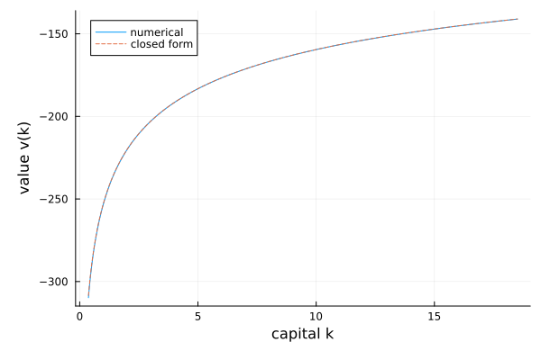

Consumption rises with capital (left). The capital drift $\mu_k$ (right) is positive below the steady state and negative above it, crossing zero exactly at $\bar k$ — the saddle-path-stable steady state the economy is drawn toward.

p1 = plot(ks, result.saved.c; xlabel = "capital k", ylabel = "consumption c(k)",
          label = "numerical")
plot!(p1, ks, c_closed; linestyle = :dash, label = "closed form")
p2 = plot(ks, result.saved.μk; xlabel = "capital k", ylabel = "capital drift μk", legend = false)
hline!(p2, [0.0]; color = :gray, linestyle = :dash)
vline!(p2, [k̄]; color = :red, linestyle = :dot)
plot(p1, p2; layout = (1, 2), size = (800, 300))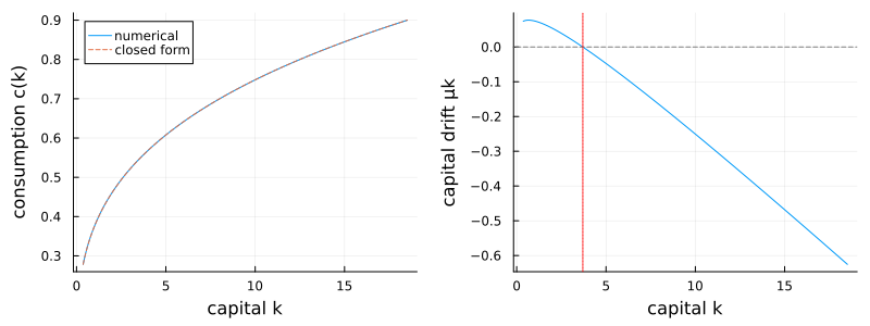

This page was generated using Literate.jl.