Gârleanu–Panageas with long-run risk: values backward, prices forward

This example solves a heterogeneous-agent a la Gârleanu–Panageas economy but where the aggregate endowment process has long-run-risk dynamics. There are now three state variables: x, the type-A consumption share; μ, expected endowment growth; and v, the conditional variance of endowment growth.

To my knowledge, no one has ever discussed such a model –- one reason being that that it is hard to solve models on a 3D state grid. The example presents a helpful solution method: formulate the model in EconPDEs by treating the interest rate and prices of risk as state-dependent unknown functions, and solve the joint system in one continuation that marches the valuation equations backward in pseudo-time and relaxes the market-clearing equations forward (tâtonnement), using a signed per-unknown time step Δ.

This example illustrates a useful way to write general-equilibrium asset-pricing systems. Rather than first solving the equilibrium pricing equations for the interest rate and prices of risk as functions of the value functions, we keep those prices as unknown functions on the grid. The unknown is

(pA, pB, ϕ1, ϕ2, r, κC, κM, κV)

where the first four entries are valuation functions and the last four are state-dependent equilibrium price functions. Their equations are algebraic restrictions: the supplied r, κC, κM, and κV must equal the values implied by market clearing at that state.

This formulation is often better conditioned than eliminating prices. In a simple one-dimensional model, substituting the equilibrium r(V) and κ(V) formulas directly into the HJB can simplify the system. In higher-dimensional models with several prices of risk, the same substitution makes the PDE operator much more nonlinear: prices affect consumption volatilities, the wealth-share drift, upwind directions, and cross derivatives. Keeping prices as algebraic unknowns makes the system larger but cleaner: optimization equations and market-clearing equations are solved simultaneously.

The same trick can be useful in other asset-pricing models whenever endogenous prices, risk premia, or volatilities feed back strongly into the law of motion. It is not needed in every model: when the equilibrium prices have simple closed forms and substituting them leaves a well-conditioned HJB, the shorter reduced-form PDE is preferable.

using EconPDEs
using Distributions
using Plots

struct GarleanuPanageasLongRunRiskModel
    γA::Float64
    ψA::Float64
    γB::Float64
    ψB::Float64
    ρ::Float64
    δ::Float64
    νA::Float64
    μbar::Float64
    vbar::Float64
    κμ::Float64
    νμ::Float64
    κv::Float64
    νv::Float64
    B1::Float64
    δ1::Float64
    B2::Float64
    δ2::Float64
    ω::Float64
end

function GarleanuPanageasLongRunRiskModel(;
        γA = 1.5, ψA = 0.7, γB = 10.0, ψB = 0.05, ρ = 0.001,
        δ = 0.02, νA = 0.01, μbar = 0.018, vbar = 0.00073,
        κμ = 0.252, νμ = 0.528, κv = 0.156, νv = 0.00354,
        B1 = 30.72, δ1 = 0.0525, B2 = -30.29, δ2 = 0.0611,
        ω = 0.92)

    scale = δ / (δ + δ1) * B1 + δ / (δ + δ2) * B2
    return GarleanuPanageasLongRunRiskModel(γA, ψA, γB, ψB, ρ, δ,
        νA, μbar, vbar, κμ, νμ, κv, νv, B1 / scale, δ1, B2 / scale, δ2, ω)
end

function (model::GarleanuPanageasLongRunRiskModel)(state::NamedTuple, u::NamedTuple)
    (; γA, ψA, γB, ψB, ρ, δ, νA, μbar, vbar, κμ, νμ, κv, νv, B1, δ1, B2, δ2, ω) = model
    (; x, μ, v) = state

    pA, pB, ϕ1, ϕ2 = u.pA, u.pB, u.ϕ1, u.ϕ2
    r, κC, κM, κV = u.r, u.κC, u.κM, u.κV

    σc = sqrt(v)
    μμ = κμ * (μbar - μ)
    σμ = νμ * sqrt(v)
    μv = κv * (vbar - v)
    σv = νv * sqrt(v)

    pAμ = (μμ >= 0) ? u.pAμ_up : u.pAμ_down
    pBμ = (μμ >= 0) ? u.pBμ_up : u.pBμ_down
    ϕ1μ = (μμ >= 0) ? u.ϕ1μ_up : u.ϕ1μ_down
    ϕ2μ = (μμ >= 0) ? u.ϕ2μ_up : u.ϕ2μ_down
    pAv = (μv >= 0) ? u.pAv_up : u.pAv_down
    pBv = (μv >= 0) ? u.pBv_up : u.pBv_down
    ϕ1v = (μv >= 0) ? u.ϕ1v_up : u.ϕ1v_down
    ϕ2v = (μv >= 0) ? u.ϕ2v_up : u.ϕ2v_down

    pAx, pBx, ϕ1x, ϕ2x = u.pAx_up, u.pBx_up, u.ϕ1x_up, u.ϕ2x_up
    iter = 0
    μx = 0.0
    σxC = 0.0
    σxM = 0.0
    σxV = 0.0
    σCA_C = 0.0
    σCA_M = 0.0
    σCA_V = 0.0
    σCB_C = 0.0
    σCB_M = 0.0
    σCB_V = 0.0
    κ2 = 0.0
    mcA = 0.0
    mcB = 0.0
    @label start

    Γ = 1 / (x / γA + (1 - x) / γB)
    aA = (1 - γA * ψA) / (γA * (ψA - 1))
    aB = (1 - γB * ψB) / (γB * (ψB - 1))

    pAx_pA = pAx / pA
    pBx_pB = pBx / pB
    pAμ_pA = pAμ / pA
    pBμ_pB = pBμ / pB
    pAv_pA = pAv / pA
    pBv_pB = pBv / pB

    denom = 1 - x * aA * pAx_pA
    σxC = x * (κC / γA - σc) / denom
    σxM = x * (κM / γA + aA * pAμ_pA * σμ) / denom
    σxV = x * (κV / γA + aA * pAv_pA * σv) / denom
    σx2 = σxC^2 + σxM^2 + σxV^2

    σpA_C = pAx_pA * σxC
    σpA_M = pAx_pA * σxM + pAμ_pA * σμ
    σpA_V = pAx_pA * σxV + pAv_pA * σv
    σpB_C = pBx_pB * σxC
    σpB_M = pBx_pB * σxM + pBμ_pB * σμ
    σpB_V = pBx_pB * σxV + pBv_pB * σv

    σCA_C = κC / γA + aA * σpA_C
    σCA_M = κM / γA + aA * σpA_M
    σCA_V = κV / γA + aA * σpA_V
    σCB_C = κC / γB + aB * σpB_C
    σCB_M = κM / γB + aB * σpB_M
    σCB_V = κV / γB + aB * σpB_V

    κ2 = κC^2 + κM^2 + κV^2
    σpA2 = σpA_C^2 + σpA_M^2 + σpA_V^2
    σpB2 = σpB_C^2 + σpB_M^2 + σpB_V^2
    κσpA = κC * σpA_C + κM * σpA_M + κV * σpA_V
    κσpB = κC * σpB_C + κM * σpB_M + κV * σpB_V
    mcA = (1 + ψA) / (2 * γA) * κ2 + aA * κσpA - 0.5 * aA * σpA2
    mcB = (1 + ψB) / (2 * γB) * κ2 + aB * κσpB - 0.5 * aB * σpB2

    human_capital = ω * (B1 * ϕ1 + B2 * ϕ2)
    μCA = ψA * (r - ρ) + mcA
    μCB = ψB * (r - ρ) + mcB
    μx = x * (μCA - μ) + δ * (νA / pA * human_capital - x) - σc * σxC

    if (iter == 0) && (μx <= 0)
        iter += 1
        pAx, pBx, ϕ1x, ϕ2x = u.pAx_down, u.pBx_down, u.ϕ1x_down, u.ϕ2x_down
        @goto start
    end

    pAxμ = (σxM * σμ >= 0) ? u.pAxμ_up : u.pAxμ_down
    pBxμ = (σxM * σμ >= 0) ? u.pBxμ_up : u.pBxμ_down
    ϕ1xμ = (σxM * σμ >= 0) ? u.ϕ1xμ_up : u.ϕ1xμ_down
    ϕ2xμ = (σxM * σμ >= 0) ? u.ϕ2xμ_up : u.ϕ2xμ_down
    pAxv = (σxV * σv >= 0) ? u.pAxv_up : u.pAxv_down
    pBxv = (σxV * σv >= 0) ? u.pBxv_up : u.pBxv_down
    ϕ1xv = (σxV * σv >= 0) ? u.ϕ1xv_up : u.ϕ1xv_down
    ϕ2xv = (σxV * σv >= 0) ? u.ϕ2xv_up : u.ϕ2xv_down

    ϕ1x_ϕ1 = ϕ1x / ϕ1
    ϕ2x_ϕ2 = ϕ2x / ϕ2
    ϕ1μ_ϕ1 = ϕ1μ / ϕ1
    ϕ2μ_ϕ2 = ϕ2μ / ϕ2
    ϕ1v_ϕ1 = ϕ1v / ϕ1
    ϕ2v_ϕ2 = ϕ2v / ϕ2

    σϕ1_C = ϕ1x_ϕ1 * σxC
    σϕ1_M = ϕ1x_ϕ1 * σxM + ϕ1μ_ϕ1 * σμ
    σϕ1_V = ϕ1x_ϕ1 * σxV + ϕ1v_ϕ1 * σv
    σϕ2_C = ϕ2x_ϕ2 * σxC
    σϕ2_M = ϕ2x_ϕ2 * σxM + ϕ2μ_ϕ2 * σμ
    σϕ2_V = ϕ2x_ϕ2 * σxV + ϕ2v_ϕ2 * σv

    μpA = pAx_pA * μx + pAμ_pA * μμ + pAv_pA * μv +
          0.5 * u.pAxx / pA * σx2 + 0.5 * u.pAμμ / pA * σμ^2 +
          0.5 * u.pAvv / pA * σv^2 + pAxμ / pA * σxM * σμ +
          pAxv / pA * σxV * σv
    μpB = pBx_pB * μx + pBμ_pB * μμ + pBv_pB * μv +
          0.5 * u.pBxx / pB * σx2 + 0.5 * u.pBμμ / pB * σμ^2 +
          0.5 * u.pBvv / pB * σv^2 + pBxμ / pB * σxM * σμ +
          pBxv / pB * σxV * σv
    μϕ1 = ϕ1x_ϕ1 * μx + ϕ1μ_ϕ1 * μμ + ϕ1v_ϕ1 * μv +
          0.5 * u.ϕ1xx / ϕ1 * σx2 + 0.5 * u.ϕ1μμ / ϕ1 * σμ^2 +
          0.5 * u.ϕ1vv / ϕ1 * σv^2 + ϕ1xμ / ϕ1 * σxM * σμ +
          ϕ1xv / ϕ1 * σxV * σv
    μϕ2 = ϕ2x_ϕ2 * μx + ϕ2μ_ϕ2 * μμ + ϕ2v_ϕ2 * μv +
          0.5 * u.ϕ2xx / ϕ2 * σx2 + 0.5 * u.ϕ2μμ / ϕ2 * σμ^2 +
          0.5 * u.ϕ2vv / ϕ2 * σv^2 + ϕ2xμ / ϕ2 * σxM * σμ +
          ϕ2xv / ϕ2 * σxV * σv

    σCAσpA = σCA_C * σpA_C + σCA_M * σpA_M + σCA_V * σpA_V
    σCBσpB = σCB_C * σpB_C + σCB_M * σpB_M + σCB_V * σpB_V
    κσpA_CA = κC * (σpA_C + σCA_C) + κM * (σpA_M + σCA_M) +
              κV * (σpA_V + σCA_V)
    κσpB_CB = κC * (σpB_C + σCB_C) + κM * (σpB_M + σCB_M) +
              κV * (σpB_V + σCB_V)

    pAt = -pA * (1 / pA + μCA + μpA + σCAσpA - r - δ - κσpA_CA)
    pBt = -pB * (1 / pB + μCB + μpB + σCBσpB - r - δ - κσpB_CB)

    κσϕ1_Y = κC * (σϕ1_C + σc) + κM * σϕ1_M + κV * σϕ1_V
    κσϕ2_Y = κC * (σϕ2_C + σc) + κM * σϕ2_M + κV * σϕ2_V
    ϕ1t = -ϕ1 * (1 / ϕ1 + μ - δ - δ1 + μϕ1 + σc * σϕ1_C - r - κσϕ1_Y)
    ϕ2t = -ϕ2 * (1 / ϕ2 + μ - δ - δ2 + μϕ2 + σc * σϕ2_C - r - κσϕ2_Y)

    κC_implied = Γ * (σc - x * aA * σpA_C - (1 - x) * aB * σpB_C)
    κM_implied = Γ * (0.0 - x * aA * σpA_M - (1 - x) * aB * σpB_M)
    κV_implied = Γ * (0.0 - x * aA * σpA_V - (1 - x) * aB * σpB_V)
    r_implied = ρ + (μ - x * mcA - (1 - x) * mcB -
                δ * ((νA / pA + (1 - νA) / pB) * human_capital - 1)) /
                (ψA * x + ψB * (1 - x))

    # The market-clearing equations are written in their natural forward (tâtonnement)
    # direction: the residual is positive when the implied price exceeds the current
    # guess, so the price converges by marching *forward* in pseudo-time. The valuation
    # equations above are backward equations instead (hence their leading minus). The
    # signed `Δ` passed to `pdesolve` below encodes this per unknown: negative time
    # steps for the price functions, positive for the valuation functions.
    rt = r_implied - r
    κCt = κC_implied - κC
    κMt = κM_implied - κM
    κVt = κV_implied - κV

    return (; pAt, pBt, ϕ1t, ϕ2t, rt, κCt, κMt, κVt),
           (; κ = sqrt(κ2), r_implied, κC_implied, κM_implied, κV_implied,
              r_gap = rt, κC_gap = κCt, κM_gap = κMt, κV_gap = κVt,
              pA_residual = pAt, pB_residual = pBt,
              ϕ1_residual = ϕ1t, ϕ2_residual = ϕ2t,
              μx, σx = sqrt(σx2), σxC, σxM, σxV)
end

Define the state grid and the initial guess for value functions and equilibrium price functions.

function initialize_stategrid(m::GarleanuPanageasLongRunRiskModel;
        xn = 20, μn = 5, vn = 5)
    μsd = sqrt(m.νμ^2 * m.vbar / (2 * m.κμ))
    μdistribution = Normal(m.μbar, μsd)
    vdistribution = Gamma(2 * m.κv * m.vbar / m.νv^2, m.νv^2 / (2 * m.κv))
    return (; x = collect(range(0.0, 1.0, length = xn).^2),
            μ = collect(range(quantile(μdistribution, 0.10),
                              quantile(μdistribution, 0.90), length = μn)),
            v = collect(range(quantile(vdistribution, 0.10),
                              quantile(vdistribution, 0.90), length = vn)))
end

function initialize_guess(m::GarleanuPanageasLongRunRiskModel, stategrid)
    gridsize = map(length, values(stategrid))
    pA = ones(gridsize...)
    pB = ones(gridsize...)
    ϕ1 = ones(gridsize...)
    ϕ2 = ones(gridsize...)
    r = zeros(gridsize...)
    κC = zeros(gridsize...)
    κM = zeros(gridsize...)
    κV = zeros(gridsize...)
    human_capital = m.ω * (m.B1 + m.B2)
    for (ix, x) in pairs(stategrid.x), (iμ, μ) in pairs(stategrid.μ), (iv, v) in pairs(stategrid.v)
        σc = sqrt(v)
        Γ = 1 / (x / m.γA + (1 - x) / m.γB)
        κC[ix, iμ, iv] = Γ * σc
        κ2 = κC[ix, iμ, iv]^2
        mcA = (1 + m.ψA) / (2 * m.γA) * κ2
        mcB = (1 + m.ψB) / (2 * m.γB) * κ2
        r[ix, iμ, iv] = m.ρ + (μ - x * mcA - (1 - x) * mcB -
                          m.δ * (human_capital - 1)) / (m.ψA * x + m.ψB * (1 - x))
    end
    return (; pA, pB, ϕ1, ϕ2, r, κC, κM, κV)
end

m = GarleanuPanageasLongRunRiskModel()
stategrid = initialize_stategrid(m)
guess = initialize_guess(m, stategrid)

(pA = [1.0 1.0 … 1.0 1.0; 1.0 1.0 … 1.0 1.0; … ; 1.0 1.0 … 1.0 1.0; 1.0 1.0 … 1.0 1.0;;; 1.0 1.0 … 1.0 1.0; 1.0 1.0 … 1.0 1.0; … ; 1.0 1.0 … 1.0 1.0; 1.0 1.0 … 1.0 1.0;;; 1.0 1.0 … 1.0 1.0; 1.0 1.0 … 1.0 1.0; … ; 1.0 1.0 … 1.0 1.0; 1.0 1.0 … 1.0 1.0;;; 1.0 1.0 … 1.0 1.0; 1.0 1.0 … 1.0 1.0; … ; 1.0 1.0 … 1.0 1.0; 1.0 1.0 … 1.0 1.0;;; 1.0 1.0 … 1.0 1.0; 1.0 1.0 … 1.0 1.0; … ; 1.0 1.0 … 1.0 1.0; 1.0 1.0 … 1.0 1.0], pB = [1.0 1.0 … 1.0 1.0; 1.0 1.0 … 1.0 1.0; … ; 1.0 1.0 … 1.0 1.0; 1.0 1.0 … 1.0 1.0;;; 1.0 1.0 … 1.0 1.0; 1.0 1.0 … 1.0 1.0; … ; 1.0 1.0 … 1.0 1.0; 1.0 1.0 … 1.0 1.0;;; 1.0 1.0 … 1.0 1.0; 1.0 1.0 … 1.0 1.0; … ; 1.0 1.0 … 1.0 1.0; 1.0 1.0 … 1.0 1.0;;; 1.0 1.0 … 1.0 1.0; 1.0 1.0 … 1.0 1.0; … ; 1.0 1.0 … 1.0 1.0; 1.0 1.0 … 1.0 1.0;;; 1.0 1.0 … 1.0 1.0; 1.0 1.0 … 1.0 1.0; … ; 1.0 1.0 … 1.0 1.0; 1.0 1.0 … 1.0 1.0], ϕ1 = [1.0 1.0 … 1.0 1.0; 1.0 1.0 … 1.0 1.0; … ; 1.0 1.0 … 1.0 1.0; 1.0 1.0 … 1.0 1.0;;; 1.0 1.0 … 1.0 1.0; 1.0 1.0 … 1.0 1.0; … ; 1.0 1.0 … 1.0 1.0; 1.0 1.0 … 1.0 1.0;;; 1.0 1.0 … 1.0 1.0; 1.0 1.0 … 1.0 1.0; … ; 1.0 1.0 … 1.0 1.0; 1.0 1.0 … 1.0 1.0;;; 1.0 1.0 … 1.0 1.0; 1.0 1.0 … 1.0 1.0; … ; 1.0 1.0 … 1.0 1.0; 1.0 1.0 … 1.0 1.0;;; 1.0 1.0 … 1.0 1.0; 1.0 1.0 … 1.0 1.0; … ; 1.0 1.0 … 1.0 1.0; 1.0 1.0 … 1.0 1.0], ϕ2 = [1.0 1.0 … 1.0 1.0; 1.0 1.0 … 1.0 1.0; … ; 1.0 1.0 … 1.0 1.0; 1.0 1.0 … 1.0 1.0;;; 1.0 1.0 … 1.0 1.0; 1.0 1.0 … 1.0 1.0; … ; 1.0 1.0 … 1.0 1.0; 1.0 1.0 … 1.0 1.0;;; 1.0 1.0 … 1.0 1.0; 1.0 1.0 … 1.0 1.0; … ; 1.0 1.0 … 1.0 1.0; 1.0 1.0 … 1.0 1.0;;; 1.0 1.0 … 1.0 1.0; 1.0 1.0 … 1.0 1.0; … ; 1.0 1.0 … 1.0 1.0; 1.0 1.0 … 1.0 1.0;;; 1.0 1.0 … 1.0 1.0; 1.0 1.0 … 1.0 1.0; … ; 1.0 1.0 … 1.0 1.0; 1.0 1.0 … 1.0 1.0], r = [0.03375388192964305 0.29127696901909944 … 0.8063231431980123 1.0638462302874687; 0.03284626663607571 0.28141801647375964 … 0.7785615161491274 1.027133265986811; … ; 0.00676232745258274 0.02709161554339704 … 0.06775019172502564 0.08807947981583993; 0.00629777409026621 0.024692280310941672 … 0.061481292752292596 0.07987579897296805;;; 0.02232739463444878 0.27985048172390525 … 0.7948966559028182 1.0524197429922744; 0.021865188777569714 0.2704369386152536 … 0.7675804382906214 1.016152188128305; … ; 0.006523903474285043 0.026853191565099337 … 0.06751176774672793 0.08784105583754225; 0.006099559514737328 0.024494065735412796 … 0.06128307817676372 0.07967758439743917;;; 0.010900907339254508 0.2684239944287109 … 0.7834701686076238 1.0409932556970802; 0.010884110919063682 0.25945586075674754 … 0.7565993604321152 1.005171110269799; … ; 0.006285479495987343 0.02661476758680164 … 0.06727334376843022 0.08760263185924455; 0.005901344939208449 0.024295851159883912 … 0.061084863601234836 0.0794793698219103;;; -0.0005255799559397987 0.25699750713351666 … 0.7720436813124295 1.0295667684018859; -9.696693944238628e-5 0.24847478289824151 … 0.7456182825736093 0.9941900324112932; … ; 0.006047055517689644 0.026376343608503945 … 0.06703491979013253 0.08736420788094684; 0.005703130363679568 0.024097636584355032 … 0.060886649025705945 0.07928115524638142;;; -0.011952067251134034 0.24557101983832239 … 0.7606171940172353 1.0181402811066915; -0.011078044797948387 0.2374937050397355 … 0.7346372047151032 0.983208954552787; … ; 0.005808631539391944 0.02613791963020624 … 0.06679649581183483 0.08712578390264913; 0.005504915788150689 0.02389942200882615 … 0.06068843445017707 0.07908294067085254], κC = [0.22824172151274014 0.22824172151274014 … 0.22824172151274014 0.22824172151274014; 0.2247143494529978 0.2247143494529978 … 0.2247143494529978 0.2247143494529978; … ; 0.03750353275653127 0.03750353275653127 … 0.03750353275653127 0.03750353275653127; 0.03423625822691102 0.03423625822691102 … 0.03423625822691102 0.03423625822691102;;; 0.25095149390203914 0.25095149390203914 … 0.25095149390203914 0.25095149390203914; 0.247073152632644 0.247073152632644 … 0.247073152632644 0.247073152632644; … ; 0.04123508843815937 0.04123508843815937 … 0.04123508843815937 0.04123508843815937; 0.037642724085305876 0.037642724085305876 … 0.037642724085305876 0.037642724085305876;;; 0.2717701623508938 0.2717701623508938 … 0.2717701623508938 0.2717701623508938; 0.26757007802365274 0.26757007802365274 … 0.26757007802365274 0.26757007802365274; … ; 0.04465590742315552 0.04465590742315552 … 0.04465590742315552 0.04465590742315552; 0.04076552435263407 0.04076552435263407 … 0.04076552435263407 0.04076552435263407;;; 0.29110374438814274 0.29110374438814274 … 0.29110374438814274 0.29110374438814274; 0.28660486833850785 0.28660486833850785 … 0.28660486833850785 0.28660486833850785; … ; 0.04783270447160653 0.04783270447160653 … 0.04783270447160653 0.04783270447160653; 0.04366556165822141 0.04366556165822141 … 0.04366556165822141 0.04366556165822141;;; 0.30923091509317613 0.30923091509317613 … 0.30923091509317613 0.30923091509317613; 0.304451891859918 0.304451891859918 … 0.304451891859918 0.304451891859918; … ; 0.05081127007220601 0.05081127007220601 … 0.05081127007220601 0.05081127007220601; 0.04638463726397642 0.04638463726397642 … 0.04638463726397642 0.04638463726397642], κM = [0.0 0.0 … 0.0 0.0; 0.0 0.0 … 0.0 0.0; … ; 0.0 0.0 … 0.0 0.0; 0.0 0.0 … 0.0 0.0;;; 0.0 0.0 … 0.0 0.0; 0.0 0.0 … 0.0 0.0; … ; 0.0 0.0 … 0.0 0.0; 0.0 0.0 … 0.0 0.0;;; 0.0 0.0 … 0.0 0.0; 0.0 0.0 … 0.0 0.0; … ; 0.0 0.0 … 0.0 0.0; 0.0 0.0 … 0.0 0.0;;; 0.0 0.0 … 0.0 0.0; 0.0 0.0 … 0.0 0.0; … ; 0.0 0.0 … 0.0 0.0; 0.0 0.0 … 0.0 0.0;;; 0.0 0.0 … 0.0 0.0; 0.0 0.0 … 0.0 0.0; … ; 0.0 0.0 … 0.0 0.0; 0.0 0.0 … 0.0 0.0], κV = [0.0 0.0 … 0.0 0.0; 0.0 0.0 … 0.0 0.0; … ; 0.0 0.0 … 0.0 0.0; 0.0 0.0 … 0.0 0.0;;; 0.0 0.0 … 0.0 0.0; 0.0 0.0 … 0.0 0.0; … ; 0.0 0.0 … 0.0 0.0; 0.0 0.0 … 0.0 0.0;;; 0.0 0.0 … 0.0 0.0; 0.0 0.0 … 0.0 0.0; … ; 0.0 0.0 … 0.0 0.0; 0.0 0.0 … 0.0 0.0;;; 0.0 0.0 … 0.0 0.0; 0.0 0.0 … 0.0 0.0; … ; 0.0 0.0 … 0.0 0.0; 0.0 0.0 … 0.0 0.0;;; 0.0 0.0 … 0.0 0.0; 0.0 0.0 … 0.0 0.0; … ; 0.0 0.0 … 0.0 0.0; 0.0 0.0 … 0.0 0.0])

Solving jointly: values backward, prices forward

The eight equations have two natures. The four valuation equations are backward equations: discounting makes their false transient stable when marched backward in pseudo-time, which is EconPDEs' baseline convention (and the reason for the leading minus in pAt, pBt, ϕ1t, ϕ2t). The four market-clearing equations are written in the natural tâtonnement direction, rt = r_implied - r: the price adjusts forward toward the value implied by market clearing.

A signed per-unknown Δ expresses exactly this: positive entries march an equation backward, negative entries forward, and the magnitudes set relative speeds. Two choices matter here.

• Prices need damping. The feedback loop from the prices of risk to the wealth-share volatility to the valuation-ratio volatilities and back to the implied prices of risk is strong (type-B agents are very risk averse), so undamped market clearing overshoots. Δ = -1 moves each price halfway toward its implied value per step — an implicit, damped tâtonnement.
• Values can move much faster than prices. Given prices, the valuation block is a well-behaved system of parabolic equations, so it gets a time step 100 times larger: each pseudo-time step solves the valuation equations essentially exactly at the current prices, jointly with the damped price update.

The Δ entries fix a relative profile; the continuation scales all of them by one common adaptive factor. Left alone, that factor grows after every successful step, so the damping fades and the iteration turns into full Newton on the whole system. On fine grids that is premature: the price feedback loop becomes locally expansive (on this model around xn = 50), undamped market-clearing steps far from the solution fail, and the continuation wastes dozens of iterations thrashing between step sizes. We therefore solve in two stages.

1. A capped continuation (maxΔ = 3): the adaptive factor may not grow beyond 3, so the price step stays damped throughout. An implicit damped step converges even where the feedback is too strong for explicit price updates — but only linearly, so tight tolerances would be slow. We stop at a loose abstol = 1e-5.
2. A single undamped Newton solve (Δ = Inf) from the stage-1 iterate. Newton's basin of attraction is far larger than the 1e-5 handoff requires (a trust-region solve converges from market-clearing gaps of order 1e-2), and it finishes at machine precision in a handful of iterations.

None of these numbers is delicate: value steps from 10 to 1000, price steps from -0.1 to -10, and caps from 1 to 10 all converge, on grids from 10×5×5 to 100×5×5 and beyond.

Δprofile = (; pA = 100.0, pB = 100.0, ϕ1 = 100.0, ϕ2 = 100.0,
            r = -1.0, κC = -1.0, κM = -1.0, κV = -1.0)

# stage 1 — capped damped continuation: robust from the analytical guess
stage1 = pdesolve(m, stategrid, guess; Δ = Δprofile, maxΔ = 3.0,
                  abstol = 1e-5, maxiters = 100)

# stage 2 — undamped Newton polish: quadratic finish from the loose handoff
result = pdesolve(m, stategrid, stage1.solution; Δ = Inf,
                  alg = NonlinearSolve.TrustRegion(), maxiters = 100)

EconPDEResult
  solution:      pA (20×5×5), pB (20×5×5), ϕ1 (20×5×5), ϕ2 (20×5×5), r (20×5×5), κC (20×5×5), κM (20×5×5), κV (20×5×5)
  saved:         pA, pB, ϕ1, ϕ2, r, κC, κM, κV, κ, r_implied, κC_implied, κM_implied, κV_implied, r_gap, κC_gap, κM_gap, κV_gap, pA_residual, pB_residual, ϕ1_residual, ϕ2_residual, μx, σx, σxC, σxM, σxV
  residual_norm: 6.61e-14
  converged:     true (tolerance 1.49e-08)

The solution

The model has three state variables, so we inspect one-dimensional slices of the equilibrium price schedules. First vary expected growth $\mu$ while holding variance fixed at the middle grid point. Then vary variance $v$ while holding expected growth fixed at the middle grid point. The total price of risk is $\kappa = \sqrt{\kappa_C^2 + \kappa_\mu^2 + \kappa_v^2}$.

xgrid = stategrid.x
μ_mid_index = cld(length(stategrid.μ), 2)
v_mid_index = cld(length(stategrid.v), 2)
μ_indices = unique([1, μ_mid_index, length(stategrid.μ)])
v_indices = unique([1, v_mid_index, length(stategrid.v)])

r_by_μ = plot(; xlabel = "type-A consumption share x", ylabel = "interest rate r")
κ_by_μ = plot(; xlabel = "type-A consumption share x", ylabel = "total price of risk κ")
for iμ in μ_indices
    label = "μ = $(round(stategrid.μ[iμ]; digits = 3))"
    plot!(r_by_μ, xgrid, result.solution.r[:, iμ, v_mid_index]; label)
    plot!(κ_by_μ, xgrid, result.saved.κ[:, iμ, v_mid_index]; label)
end
plot(r_by_μ, κ_by_μ; layout = (1, 2), size = (820, 300))

r_by_v = plot(; xlabel = "type-A consumption share x", ylabel = "interest rate r")
κ_by_v = plot(; xlabel = "type-A consumption share x", ylabel = "total price of risk κ")
for iv in v_indices
    label = "v = $(round(stategrid.v[iv]; sigdigits = 3))"
    plot!(r_by_v, xgrid, result.solution.r[:, μ_mid_index, iv]; label)
    plot!(κ_by_v, xgrid, result.saved.κ[:, μ_mid_index, iv]; label)
end
plot(r_by_v, κ_by_v; layout = (1, 2), size = (820, 300))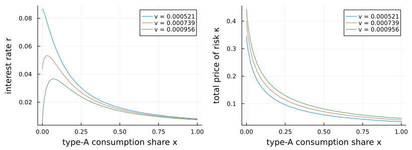

This page was generated using Literate.jl.