Gârleanu–Panageas (2015): heterogeneous agents

This is the package's most demanding kind of problem: a general-equilibrium model with endogenous volatility and several coupled value functions. Two types of agents differ in risk aversion and elasticity of intertemporal substitution — type A is "bold" (low $\gamma_A$), type B "conservative" (high $\gamma_B$). The single state $x$ is the consumption share of type A. Four claims are priced jointly: the wealth–consumption ratios $p_A, p_B$ of the two agents and two human-capital claims $\phi_1, \phi_2$.

What makes it hard is that the volatility of the state, $\sigma_x$, is endogenous — it depends on the very derivatives $p_A', p_B'$ we are solving for — so the upwind direction must be recomputed from the resulting drift $\mu_x$ each iteration.

Defining the model

The parameters:

using EconPDEs, Plots

Base.@kwdef struct GarleanuPanageasModel
    γA::Float64 = 1.5      # relative risk aversion, type A (bold)
    ψA::Float64 = 0.7      # elasticity of intertemporal substitution, type A
    γB::Float64 = 10.0     # relative risk aversion, type B (conservative)
    ψB::Float64 = 0.05     # elasticity of intertemporal substitution, type B
    ρ::Float64 = 0.001     # rate of time preference (discount rate)
    δ::Float64 = 0.02      # death (turnover) rate
    νA::Float64 = 0.01     # share of type A among newborns
    μ::Float64 = 0.02      # aggregate consumption growth (drift)
    σ::Float64 = 0.041     # aggregate consumption volatility
    B1::Float64 = 30.72    # loading on first component of labor-income profile
    δ1::Float64 = 0.0525   # decay rate of first labor-income component
    B2::Float64 = -30.29   # loading on second component of labor-income profile
    δ2::Float64 = 0.0611   # decay rate of second labor-income component
    ω::Float64 = 0.92      # labor share of aggregate output
    function GarleanuPanageasModel(γA, ψA, γB, ψB, ρ, δ, νA, μ, σ, B1, δ1, B2, δ2, ω)
        # Normalize the labor-income loadings once, at construction, so the newborn's human capital is one.
        scale = δ / (δ + δ1) * B1 + δ / (δ + δ2) * B2
        new(γA, ψA, γB, ψB, ρ, δ, νA, μ, σ, B1 / scale, δ1, B2 / scale, δ2, ω)
    end
end

Main.GarleanuPanageasModel

We solve the model at its default parameters:

m = GarleanuPanageasModel()

Main.GarleanuPanageasModel(1.5, 0.7, 10.0, 0.05, 0.001, 0.02, 0.01, 0.02, 0.041, 30.57652344371571, 0.0525, -30.148531741866826, 0.0611, 0.92)

Defining the grid

We define the grid, a NamedTuple keyed by the state variable $x$, the consumption share of type A, on $[0, 1]$.

stategrid = (; x = range(0.0, 1.0, length = 100))

(x = 0.0:0.010101010101010102:1.0,)

Defining an initial guess

We define the initial guess, a NamedTuple whose keys are the four coupled unknown functions (pA, pB, ϕ1, ϕ2), all initialized flat at one. These names — and their finite differences, such as pAx_up — are what reappear inside the equation below.

guess = (; pA = ones(length(stategrid[:x])), pB = ones(length(stategrid[:x])), ϕ1 = ones(length(stategrid[:x])), ϕ2 = ones(length(stategrid[:x])))

(pA = [1.0, 1.0, 1.0, 1.0, 1.0, 1.0, 1.0, 1.0, 1.0, 1.0  …  1.0, 1.0, 1.0, 1.0, 1.0, 1.0, 1.0, 1.0, 1.0, 1.0], pB = [1.0, 1.0, 1.0, 1.0, 1.0, 1.0, 1.0, 1.0, 1.0, 1.0  …  1.0, 1.0, 1.0, 1.0, 1.0, 1.0, 1.0, 1.0, 1.0, 1.0], ϕ1 = [1.0, 1.0, 1.0, 1.0, 1.0, 1.0, 1.0, 1.0, 1.0, 1.0  …  1.0, 1.0, 1.0, 1.0, 1.0, 1.0, 1.0, 1.0, 1.0, 1.0], ϕ2 = [1.0, 1.0, 1.0, 1.0, 1.0, 1.0, 1.0, 1.0, 1.0, 1.0  …  1.0, 1.0, 1.0, 1.0, 1.0, 1.0, 1.0, 1.0, 1.0, 1.0])

Defining the PDE

We now write the function encoding the equilibrium conditions. Following the package convention, it takes the current state (a grid point) and u — the local bundle holding each unknown and its finite-difference derivatives there — and returns the time derivative of each unknown (pAt, pBt, ϕ1t, ϕ2t).

Because $\sigma_x$ is endogenous, the loop recomputes the upwind direction from the drift $\mu_x$: it starts with forward differences (*_up) and switches to backward (*_down) when the drift turns negative.

function (m::GarleanuPanageasModel)(state::NamedTuple, u::NamedTuple)
    (; γA, ψA, γB, ψB, ρ, δ, νA, μ, σ, B1, δ1, B2, δ2, ω) = m
    (; x) = state
    (; pA, pAx_up, pAx_down, pAxx, pB, pBx_up, pBx_down, pBxx, ϕ1, ϕ1x_up, ϕ1x_down, ϕ1xx, ϕ2, ϕ2x_up, ϕ2x_down, ϕ2xx) = u

    # endogenous σx depends on the unknown derivatives, so pick the upwind direction from μx
    pAx, pBx, ϕ1x, ϕ2x = pAx_up, pBx_up, ϕ1x_up, ϕ2x_up
    iter = 0
    @label start
    Γ = 1 / (x / γA + (1 - x) / γB)
    p = x * pA + (1 - x) * pB
    σx = σ * x * (Γ / γA - 1) / (1 + Γ * x * (1 - x) / (γA * γB) * ((1 - γB * ψB) / (ψB - 1) * (pBx / pB) - (1 - γA * ψA) / (ψA - 1) * (pAx / pA)))
    σpA = pAx / pA * σx
    σpB = pBx / pB * σx
    σϕ1 = ϕ1x / ϕ1 * σx
    σϕ2 = ϕ2x / ϕ2 * σx
    κ = Γ * (σ - x * (1 - γA * ψA) / (γA * (ψA - 1)) * σpA - (1 - x) * (1 - γB * ψB) / (γB * (ψB - 1)) * σpB)
    σCA = κ / γA + (1 - γA * ψA) / (γA * (ψA - 1)) * σpA
    σCB = κ / γB + (1 - γB * ψB) / (γB * (ψB - 1)) * σpB
    mcA = κ^2 * (1 + ψA) / (2 * γA) + (1 - ψA * γA) / (γA * (ψA - 1)) * κ * σpA - (1 - γA * ψA) / (2 * γA * (ψA - 1)) * σpA^2
    mcB = κ^2 * (1 + ψB) / (2 * γB) + (1 - ψB * γB) / (γB * (ψB - 1)) * κ * σpB - (1 - γB * ψB) / (2 * γB * (ψB - 1)) * σpB^2
    r = ρ + 1 / (ψA * x + ψB * (1 - x)) * (μ - x * mcA - (1 - x) * mcB - δ * ((νA / pA + (1 - νA) / pB) * ω * (B1 * ϕ1 + B2 * ϕ2) - 1))
    μCA = ψA * (r - ρ) + mcA
    μCB = ψB * (r - ρ) + mcB
    μx = x * (μCA - μ) + δ * (νA / pA * ω * (B1 * ϕ1 + B2 * ϕ2) - x) - σ * σx
    if (iter == 0) && (μx <= 0)
        iter += 1
        pAx, pBx, ϕ1x, ϕ2x = pAx_down, pBx_down, ϕ1x_down, ϕ2x_down
        @goto start
    end

    μpA = pAx / pA * μx + 0.5 * pAxx / pA * σx^2
    μpB = pBx / pB * μx + 0.5 * pBxx / pB * σx^2
    μϕ1 = ϕ1x / ϕ1 * μx + 0.5 * ϕ1xx / ϕ1 * σx^2
    μϕ2 = ϕ2x / ϕ2 * μx + 0.5 * ϕ2xx / ϕ2 * σx^2

    pAt = -pA * (1 / pA + μCA + μpA + σCA * σpA - r - δ - κ * (σpA + σCA))
    pBt = -pB * (1 / pB + μCB + μpB + σCB * σpB - r - δ - κ * (σpB + σCB))
    ϕ1t = -ϕ1 * (1 / ϕ1 + μ - δ - δ1 + μϕ1 + σ * σϕ1 - r - κ * (σϕ1 + σ))
    ϕ2t = -ϕ2 * (1 / ϕ2 + μ - δ - δ2 + μϕ2 + σ * σϕ2 - r - κ * (σϕ2 + σ))

    return (; pAt, pBt, ϕ1t, ϕ2t), (; r, κ)
end

Solving the model

With the grid, guess, and equation in hand, pdesolve solves the stationary system:

result = pdesolve(m, stategrid, guess)

EconPDEResult
  solution:      pA (100), pB (100), ϕ1 (100), ϕ2 (100)
  saved:         pA, pB, ϕ1, ϕ2, r, κ
  residual_norm: 1.43e-10
  converged:     true (tolerance 1.49e-08)

The solution

We saved the equilibrium interest rate $r$ and the price of risk $\kappa$ on the grid. The price of risk is high when the conservative agents (type B, high $\gamma$) hold most of the economy's wealth (low $x$) and falls as the bold agents (type A) come to dominate — risk is borne more willingly when the less risk-averse agents are wealthier.

xs = stategrid[:x]
p1 = plot(xs, result.saved.κ; xlabel = "consumption share of bold agents x", ylabel = "price of risk κ", legend = false)
p2 = plot(xs, result.saved.r; xlabel = "consumption share of bold agents x", ylabel = "interest rate r", legend = false)
plot(p1, p2; layout = (1, 2), size = (800, 300))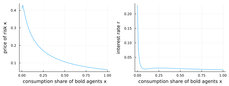

This page was generated using Literate.jl.