Wachter (2013): time-varying rare-disaster risk

Wachter asks whether a time-varying probability of rare consumption disasters can explain the high mean and volatility of the equity premium. Consumption follows a jump–diffusion: most of the time it grows smoothly, but at Poisson rate $\lambda_t$ a disaster strikes and lowers consumption by a random factor $e^{Z}$ (with $Z<0$). The single state is the disaster intensity $\lambda_t$, which mean-reverts as a square-root (CIR) process:

\[d\lambda_t = \kappa_\lambda(\bar\lambda - \lambda_t)\,dt + \nu_\lambda\sqrt{\lambda_t}\,dB_t.\]

With Epstein–Zin preferences the unknown is the wealth–consumption ratio $p(\lambda)$. Because disaster risk moves over time, so do risk premia and valuations — even though realized consumption is smooth outside disasters.

Defining the model

The parameters live in a struct:

using EconPDEs, Distributions, Plots

Base.@kwdef struct WachterModel{T<: Distribution}
    # consumption process parameters
    μ::Float64 = 0.025      # expected consumption growth
    σ::Float64 = 0.02       # volatility of consumption growth

    # disaster process parameters
    λbar::Float64 = 0.0355  # long-run mean disaster intensity
    κλ::Float64 = 0.08      # mean-reversion speed of disaster intensity
    νλ::Float64 = 0.067     # volatility of disaster intensity
    ZDistribution::T = Normal(-0.4, 0.25) # distribution of disaster jump size Z (log consumption drop); from Ian Martin higher order cumulants paper

    # utility parameters
    ρ::Float64 = 0.012      # discount rate
    γ::Float64 = 3.0        # relative risk aversion
    ψ::Float64 = 1.1        # elasticity of intertemporal substitution
    ϕ::Float64 = 2.6        # leverage of dividends on consumption
end

We solve the model at its default parameters:

m = WachterModel()

Main.WachterModel{Distributions.Normal{Float64}}(0.025, 0.02, 0.0355, 0.08, 0.067, Distributions.Normal{Float64}(μ=-0.4, σ=0.25), 0.012, 3.0, 1.1, 2.6)

Defining the grid

We define the grid, a NamedTuple whose key is the state variable (λ, the disaster intensity). The state $\lambda$ ranges from zero up to well above its long-run mean $\bar\lambda$. The $\sqrt\lambda$ diffusion vanishes at $\lambda = 0$, a degenerate boundary where no condition is imposed.

function initialize_stategrid(m::WachterModel; λn = 30)
  (; λ = range(0.0, 0.1, length = λn))
end

initialize_stategrid (generic function with 1 method)

Defining an initial guess

We define the initial guess, a NamedTuple whose key is the unknown function (p, the wealth–consumption ratio). These names (and the finite differences of $p$, such as pλ_up) are what reappear in the equation below. We then build the grid and guess from the model:

function initialize_guess(m::WachterModel, stategrid)
    λn = length(stategrid[:λ])
    (; p = ones(λn))
end

stategrid = initialize_stategrid(m)
guess = initialize_guess(m, stategrid)

(p = [1.0, 1.0, 1.0, 1.0, 1.0, 1.0, 1.0, 1.0, 1.0, 1.0  …  1.0, 1.0, 1.0, 1.0, 1.0, 1.0, 1.0, 1.0, 1.0, 1.0],)

Defining the PDE

We now write the function encoding the HJB equation. Following the package convention, it takes the current state (a grid point) and u (each unknown together with its finite-difference derivatives there) and returns the time derivative of each unknown.

function (m::WachterModel)(state::NamedTuple, u::NamedTuple)
    (; μ, σ, λbar, κλ, νλ, ZDistribution, ρ, γ, ψ, ϕ) = m
    (; λ) = state
    (; p, pλ_up, pλ_down, pλλ) = u

    # drift and volatility of λ and p
    μλ = κλ * (λbar - λ)
    σλ = νλ * sqrt(λ)
    # upwind on the sign of the drift of λ
    pλ = (μλ >= 0) ? pλ_up : pλ_down
    μp = pλ / p * μλ + 0.5 * pλλ / p * σλ^2
    σp_Zλ = pλ / p * σλ

    # market prices of risk
    κ_Zc = γ * σ
    κ_Zλ = (γ * ψ - 1) / (ψ - 1) * σp_Zλ
    η =  λ * (mgf(ZDistribution, 1) - 1 + mgf(ZDistribution, -γ) - 1 - (mgf(ZDistribution, 1 - γ) - 1))

    # interest rate
    r = ρ + μ / ψ - (1 + 1 / ψ) / 2 * γ * σ^2 - λ * (mgf(ZDistribution, -γ) - 1) + (1 / ψ - γ) / (1 - γ) * λ * (mgf(ZDistribution, 1 - γ) - 1) - (γ * ψ - 1) / (2 * (ψ - 1)) * σp_Zλ^2

    # market pricing of the consumption claim
    pt = - p * (1 / p  + μ + μp + λ * (mgf(ZDistribution, 1) - 1) - r - κ_Zc * σ - κ_Zλ * σp_Zλ - η)

    return (; pt)
end

Solving the model

With the grid, guess, and equation in hand, pdesolve solves the stationary system:

result = pdesolve(m, stategrid, guess)

EconPDEResult
  solution:      p (30)
  residual_norm: 9.79e-12
  converged:     true (tolerance 1.49e-08)

The solution

The wealth–consumption ratio falls steeply as the disaster intensity $\lambda$ rises: when a disaster is more likely, the representative agent discounts the consumption claim more heavily and valuations drop.

λs = stategrid[:λ]
plot(λs, result.solution.p; xlabel = "disaster intensity λ", ylabel = "wealth–consumption ratio p", legend = false)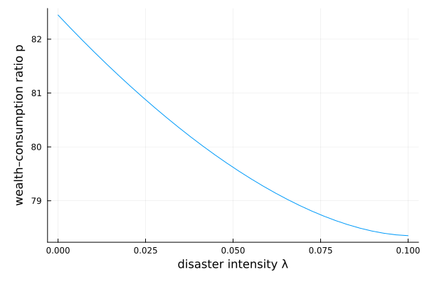

This page was generated using Literate.jl.