Brunnermeier–Sannikov (2014): a macroeconomic model with a financial sector

Experts and households both hold capital, but experts are more productive and can issue equity only if they retain at least a fraction $\chi$ of it — a skin-in-the-game constraint. The state $x$ is the experts' wealth share. The model has a crisis region (experts constrained, $\Psi < 1$) and a normal region ($\Psi = 1$). Here $\Psi$ is the share of aggregate capital operated by experts. Experts must retain the fraction $\chi$ of that operated capital, so $\chi\Psi$ is their retained capital share and $\alpha_E = \chi\Psi/x$ is capital held per unit of expert wealth. The return volatility below is $\sigma + \sigma_q$, where $\sigma_q$ is the price-revaluation term. The capital price $q$ and $\Psi$ are recovered with a bracketed root-find, sweeping $x$ from the lower boundary upward so each step reuses the previous $q$ to build $q_x$ by finite difference. That order-dependent sweep is why the model struct is mutable and carries q_old.

Defining the model

The parameters:

using EconPDEs, Roots, Plots

Base.@kwdef mutable struct BrunnermeierSannikov
  # Calibration uses Section 3.6 of the textbook chapter (the paper's r here appears to be a typo for ρH)
  ρE::Float64 = 0.06      # experts' rate of time preference (discount rate)
  ρH::Float64 = 0.05      # households' rate of time preference (discount rate)
  γ::Float64 = 2.0        # relative risk aversion
  ψ::Float64 = 0.5        # elasticity of intertemporal substitution
  δ::Float64 = 0.05       # depreciation rate of capital
  σ::Float64 = 0.1        # calibrated fundamental volatility of capital
  κ::Float64 = 10.0       # investment adjustment-cost parameter
  a::Float64 = 0.11       # experts' productivity (output per unit capital)
  alow::Float64 = 0.03    # households' productivity (output per unit capital)
  χlow::Float64 = 0.5     # minimum equity retention (skin-in-the-game floor)
  q_old::Float64 = 1.0    # previous capital price q (carried across the sweep)
  qx_old::Float64 = 0.0   # previous q_x (carried across the sweep)
  Ψ_old::Float64 = 1.0    # previous experts' capital share Ψ (carried across the sweep)
end

Main.BrunnermeierSannikov

We solve the model at its default parameters:

m = BrunnermeierSannikov()

Main.BrunnermeierSannikov(0.06, 0.05, 2.0, 0.5, 0.05, 0.1, 10.0, 0.11, 0.03, 0.5, 1.0, 0.0, 1.0)

Defining the grid

We define the grid, a NamedTuple whose key is the state variable $x$ (the experts' wealth share). The single state $x \in (0, 1)$ sits on 200 interior grid points, with the two boundaries dropped. Because the sweep marches from the lower boundary upward, the grid spacing Δx and its minimum xmin are computed here and later passed into the model.

xn = 200
stategrid =  (; x = range(0, 1.0, length = xn+2)[2:(end-1)])
Δx = step(stategrid[:x])
xmin = minimum(stategrid[:x])

0.004975124378109453

Defining an initial guess

We define the initial guess, a NamedTuple whose keys are the unknown functions (pE, pH), holding one starting value at each grid point. These names — and the finite differences of pE and pH, such as pEx_up — are what reappear inside the equation below.

guess = (; pE =  9 .* ones(xn), pH =   10 .* ones(xn))

(pE = [9.0, 9.0, 9.0, 9.0, 9.0, 9.0, 9.0, 9.0, 9.0, 9.0  …  9.0, 9.0, 9.0, 9.0, 9.0, 9.0, 9.0, 9.0, 9.0, 9.0], pH = [10.0, 10.0, 10.0, 10.0, 10.0, 10.0, 10.0, 10.0, 10.0, 10.0  …  10.0, 10.0, 10.0, 10.0, 10.0, 10.0, 10.0, 10.0, 10.0, 10.0])

Defining the PDE

A small bracketing helper locates a sign change for the crisis-region root-find below, starting from the previous step's $\Psi$:

function local_bracket(f, x0; lo = 0.0, hi = 1.0, ftol = 1e-12)
  x0 = clamp(x0, lo, hi)
  f0 = f(x0)
  isfinite(f0) || return nothing
  abs(f0) <= ftol && return (x0, x0)
  width = (hi - lo) / 64
  while width <= hi - lo
    for x1 in (min(hi, x0 + width), max(lo, x0 - width))
      f1 = f(x1)
      isfinite(f1) || continue
      abs(f1) <= ftol && return (x1, x1)
      signbit(f1) != signbit(f0) && return minmax(x0, x1)
    end
    width *= 2
  end
  return nothing
end

local_bracket (generic function with 1 method)

We now write the function encoding the equilibrium conditions. Following the package convention, it takes the current state (a grid point) and u — the local bundle holding each unknown and its finite-difference derivatives there — plus the grid spacing Δx and lower bound xmin, and returns the time derivative of each unknown (pEt, pHt). Inside, a root-find recovers the capital price $q$ and the experts' operating capital share $\Psi$, distinguishing the crisis region ($\Psi < 1$) from the normal region ($\Psi = 1$).

function (m::BrunnermeierSannikov)(state::NamedTuple, u::NamedTuple, Δx, xmin)
  (; ρE, ρH, γ, ψ, δ, σ, κ, a, alow, χlow) = m
  (; x) = state
  (; pE, pEx_up, pEx_down, pExx, pH, pHx_up, pHx_down, pHxx) = u
  # Floor the wealth–consumption ratios before dividing by them: a Newton trial iterate can wander
  # nonpositive, which would blow up the equilibrium conditions. Slack at the converged solution,
  # where both stay well above 1e-3.
  pE = max(pE, 1e-3)
  pH = max(pH, 1e-3)
  χ = max(χlow, x)
  pEx, pHx = pEx_up, pHx_up
  iter = 0
  @label start
  q_old = m.q_old
  qx_old = m.qx_old
  Ψ_old = m.Ψ_old

  # First, solve for q, qx, and qxx
  if abs(x - xmin) < 1e-9
    # initial condition at lower boundary of x grid (point outside the grid technically)
    # We must have that expert consumption approaches zero as xt approaches zero (linked to transversality condition)
    Ψ_old = 0.0
    q_old = (alow + 1 / κ) / (1 / pH + 1 / κ)
    qx_old = 0.0
  end
  if Ψ_old < 1.0
    # crisis region.
    # In this case experts operate only the share Ψ of aggregate capital. They retain χΨ of
    # aggregate capital, so their capital holding per unit of expert wealth is αE = χΨ / x.
    function crisis_gap(Ψ)
      local q = (Ψ * a + (1 - Ψ) * alow + 1 / κ) / (x / pE + (1 - x) / pH + 1 / κ)
      local qx = (q - q_old) / Δx
      local αE = χ * Ψ / x
      local σx = x * (αE - 1) * σ / (1 - x * (αE - 1) * qx / q)
      local σpE = pEx / pE * σx
      local σpH = pHx / pH * σx
      local σq = qx / q * σx
      local σE = αE * (σ + σq)
      local αH = (1 - αE * x) / (1 - x)
      local σH = αH * (σ + σq)
      local κE = γ * (σE - (1 / γ - 1) / (ψ - 1) * σpE)
      local κH = γ * (σH - (1 / γ - 1) / (ψ - 1) * σpH)
      return (a - alow) / q - χ * (κE - κH) * (σ + σq)
    end

    gap_tolerance = 1e-12
    bracket = local_bracket(crisis_gap, Ψ_old; ftol = gap_tolerance)

    if bracket === nothing
      # The unconstrained crisis equation has no root with Ψ ∈ [0, 1], so the economy is in
      # the normal region and experts operate all capital.
      Ψ_old = 1.0
    else
      Ψ = bracket[1]
      if bracket[1] != bracket[2]
        Ψ = find_zero(crisis_gap, bracket, Bisection(); xatol = gap_tolerance)
      end
      q = (Ψ * a + (1 - Ψ) * alow + 1 / κ) / (x / pE + (1 - x) / pH + 1 / κ)
      qx = (q - q_old) / Δx
    end
  end
  if Ψ_old ≥ 1.0
    # normal region.
    Ψ = 1.0
    q = (a + 1 / κ) / ((x / pE + (1 - x) / pH) + 1 / κ)
    qx = - (a + 1 / κ) / ((x / pE + (1 - x) / pH) + 1 / κ)^2 * (1 / pE - 1 / pH - x / pE^2 * pEx - (1-x) / pH^2 * pHx)
  end
  qxx = (qx - qx_old) / Δx
  m.q_old = q
  m.qx_old = qx
  m.Ψ_old = Ψ


  # having solved for q, do the time step
  # Floor q the same way before it enters ι, Φ, μq, and r; slack at the converged solution (q ≈ 1).
  q = max(q, sqrt(eps()))
  ι = (q - 1) / κ
  Φ = log(q) / κ
  αE = χ * Ψ / x
  σx = x * (αE - 1) * σ / (1 - x * (αE - 1) * qx / q)
  σpE = pEx / pE * σx
  σpH = pHx / pH * σx
  σq = qx / q * σx
  σE = αE * (σ + σq)
  αH = (1 - αE * x) / (1 - x)
  σH = αH * (σ + σq)
  κE = γ * (σE - (1 / γ - 1) / (ψ - 1) * σpE)
  κH = γ * (σH - (1 / γ - 1) / (ψ - 1) * σpH)
  μx = x * (1 - x) * (κE * σE - κH * σH + 1 / pH - 1 / pE - (σE - σH) * (σ + σq))
  μx2 = x * ((a - ι) / q - 1 / pE) + σx * (κE - σ - σq) + x * (1 - χ) * (κE - κH) * (σ + σq)
  if (iter == 0) && (μx < 0)
    # upwinding
    iter += 1
    pEx, pHx = pEx_down, pHx_down
    @goto start
  end
  μpE = pEx / pE * μx + 0.5 * pExx / pE * σx^2
  μpH = pHx / pH * μx + 0.5 * pHxx / pH * σx^2
  μq = qx / q * μx + 0.5 * qxx / q * σx^2

  # Clamp r to a wide band: a Newton trial iterate outside the economic domain can produce a wild
  # interest rate that would overflow the exponential price updates below. Slack at the converged
  # solution, where r stays within a few percent of zero.
  r = clamp((a - ι) / q + Φ - δ + μq + σ * σq - (χ * κE + (1 - χ) * κH) * (σ + σq), -3.0, 3.0)
  # Market Pricing
  pEt = -  pE * (1 / pE - ψ * ρE + (ψ - 1) * (r + κE * σE) + μpE - (ψ - 1) * γ / 2 * σE^2 + (2 - ψ - γ) / (2 * (ψ - 1)) * σpE^2 + (1 - γ) * σpE * σE)
  pHt = -  pH * (1 / pH - ψ * ρH + (ψ - 1) * (r + κH * σH) + μpH - (ψ - 1) * γ / 2 * σH^2 + (2 - ψ - γ) / (2 * (ψ - 1)) * σpH^2 + (1 - γ) * σpH * σH)
  d = Ψ * a + (1 - Ψ) * alow - ι
  μR = r + (χ * κE + (1 - χ) * κH) * (σ + σq)
  (; pEt, pHt), (; x, r, μx, σx, Ψ, κ, κE, κH, σE, σH, σq, q, qx, qxx, μq, μx2, Φ, χ, d, μR)
end

Solving the model

pdesolve solves the stationary system. Δx and xmin are passed into the model through a closure so each step of the order-dependent sweep can reuse the previous $q$:

result = pdesolve((state, u) -> m(state, u, Δx, xmin), stategrid, guess)

EconPDEResult
  solution:      pE (200), pH (200)
  saved:         pE, pH, x, r, μx, σx, Ψ, κ, κE, κH, σE, σH, σq, q, qx, qxx, μq, μx2, Φ, χ, d, μR
  residual_norm: 9.33e-11
  converged:     true (tolerance 1.49e-08)

The solution

We saved the capital price $q$. It is depressed when experts are poorly capitalized (low $x$) — the crisis region — and tends to rise with the experts' wealth share as the retention constraint slackens.

xs = stategrid[:x]
plot(xs, result.saved.q; xlabel = "experts' wealth share x", ylabel = "capital price q", legend = false)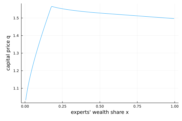

This page was generated using Literate.jl.