Haddad: concentrated ownership and endogenous volatility

This asset-pricing model has two state variables — expected consumption growth $\mu$ and consumption variance $v$ — and prices the aggregate consumption claim under Epstein–Zin preferences, much like the long-run-risk model. Its distinctive feature is concentrated ownership: only a limited set of active investors bears aggregate risk, and the equilibrium active-capital share $\alpha^\star$ is determined endogenously,

\[\alpha^\star = \bar\alpha - \sqrt{\dfrac{\lambda\,\bar\alpha}{\tfrac12\,\gamma\,\bigl(\sigma_c^2 + \sigma_{p,\mu}^2 + \sigma_{p,v}^2\bigr)}},\]

where the return-volatility terms $\sigma_{p,\mu},\sigma_{p,v}$ depend on the derivatives of the unknown price function $p(\mu, v)$. Because $\alpha^\star$ feeds the market price of risk $\kappa=\alpha^\star\gamma\sigma$ while return volatility feeds back into $\alpha^\star$, risk premia and volatility are endogenous and jointly determined. The two states themselves follow mean-reverting square-root processes.

Defining the model

The parameters live in a struct:

using EconPDEs, Distributions, Plots

Base.@kwdef struct HaddadModel
  # consumption process parameters
  μbar::Float64 = 0.018     # long-run mean of expected consumption growth μ
  vbar::Float64 = 0.00052   # long-run mean of consumption variance v
  κμ::Float64 = 0.3         # mean-reversion speed of μ
  νμ::Float64 = 0.456       # volatility loading of the μ process
  κv::Float64 = 0.012       # mean-reversion speed of v
  νv::Float64 = 0.00472     # volatility loading of the v process

  # active capital
  αbar::Float64 = 1.2       # maximum active-capital share
  λ::Float64 = 0.018        # cost of active participation (ownership friction)

  # utility parameters
  ρ::Float64 = 0.0132       # rate of time preference (discount rate)
  γ::Float64 = 10.0         # relative risk aversion
  ψ::Float64 = 1.5          # elasticity of intertemporal substitution
end

Main.HaddadModel

We solve the model at its default parameters:

m = HaddadModel()

Main.HaddadModel(0.018, 0.00052, 0.3, 0.456, 0.012, 0.00472, 1.2, 0.018, 0.0132, 10.0, 1.5)

Defining the grid

We define the grid, a NamedTuple with two keys — this model has two state variables, expected growth $\mu$ and consumption variance $v$. Each axis spans the ergodic range of its process, taken as quantiles of the stationary distribution ($\mu$ Normal, $v$ Gamma). The $\sqrt v$ diffusion vanishes at $v = 0$, a degenerate boundary where no condition is imposed.

σ = sqrt(m.νμ^2 * m.vbar / (2 * m.κμ))
μmin = quantile(Normal(m.μbar, σ), 0.001)
μmax = quantile(Normal(m.μbar, σ), 0.999)
μs = range(μmin,  μmax, length = 30)
α = 2 * m.κv * m.vbar / m.νv^2
β = m.νv^2 / (2 * m.κv)
vmin = quantile(Gamma(α, β), 0.001)
vmax = quantile(Gamma(α, β), 0.999)
vs = range(vmin,  vmax, length = 30)
stategrid = (; μ = μs, v = vs)

(μ = -0.023484132979201985:0.0028609746882208263:0.05948413297920198, v = 3.3238579690156588e-9:0.00017989085938016213:0.005216838245882671)

Defining an initial guess

We define the initial guess, a NamedTuple whose key is the single unknown function (p, the price–consumption ratio), a matrix over the $(\mu, v)$ grid initialized flat at one. This name — and its finite differences, e.g. pμ_up (forward difference in $\mu$) and pμμ (second derivative) — is what reappears inside the equation below.

guess =   (; p = ones(length(stategrid[:μ]), length(stategrid[:v])))

(p = [1.0 1.0 … 1.0 1.0; 1.0 1.0 … 1.0 1.0; … ; 1.0 1.0 … 1.0 1.0; 1.0 1.0 … 1.0 1.0],)

Defining the PDE

We now write the function encoding the HJB equation. Following the package convention, it takes the current state (a grid point) and u (each unknown together with its finite-difference derivatives there) and returns the time derivative of each unknown.

function (m::HaddadModel)(state::NamedTuple, u::NamedTuple)
  (; μbar, vbar, κμ, νμ, κv, νv, αbar, λ, ρ, γ, ψ) = m
  (; μ, v) = state
  (; p, pμ_up, pμ_down, pv_up, pv_down, pμμ, pvv) = u

  # drifts and volatilities of consumption, μ, and v
  μc = μ
  σc = sqrt(v)
  μμ = κμ * (μbar - μ)
  σμ = νμ * sqrt(v)
  μv = κv * (vbar - v)

  pμ = (μμ >= 0) ? pμ_up : pμ_down
  pv = (μv >= 0) ? pv_up : pv_down
  σv = νv * sqrt(v)
  σp_Zμ = pμ / p * σμ
  σp_Zv = pv / p * σv
  σp2 = σp_Zμ^2 + σp_Zv^2
  μp = pμ / p * μμ + pv / p * μv + 0.5 * pμμ / p * σμ^2 + 0.5 * pvv / p * σv^2

  # market price of risk, with endogenous active-capital share α*
  αstar = αbar - sqrt(λ * αbar / (0.5 * γ * (σc^2 + σp_Zμ^2 + σp_Zv^2)))
  αstar = clamp(αstar, 0.0, 1.0)
  κ_Zc = αstar * γ * σc
  κ_Zμ = (αstar - (1 / γ - 1) / (ψ - 1)) * γ * σp_Zμ
  κ_Zv = (αstar - (1 / γ - 1) / (ψ - 1)) * γ * σp_Zv
  κ2 = κ_Zc^2 + κ_Zμ^2 + κ_Zv^2

  # pricing equation for the price–consumption ratio (interest rate substituted out)
  pt = - p * (1 / p - ρ + (1 - 1 / ψ) * (μc - 0.5 * γ * σc^2 * (1 - (αstar - 1)^2)) + μp + (0.5 * (1 / ψ - γ) / (1 - 1 / ψ) + 0.5 * γ * (1 - 1 / ψ) * (αstar - 1)^2) * σp2)
  return (; pt)
end

Solving the model

With the grid, guess, and equation in hand, pdesolve solves the stationary system:

result = pdesolve(m, stategrid, guess)

EconPDEResult
  solution:      p (30×30)
  residual_norm: 1.90e-11
  converged:     true (tolerance 1.49e-08)

The solution

Holding one state fixed at its median, the price–consumption ratio rises with expected growth $\mu$ and falls with consumption variance $v$. The growth effect reflects the elasticity of intertemporal substitution ($\psi>1$): investors pay more for the claim when future growth is high. The variance effect is the risk-premium channel — and here it is amplified, because only a concentrated set of active owners bears aggregate risk, raising the effective price of risk $\alpha^\star\gamma\sigma$ and making valuations more sensitive to volatility than under full risk sharing.

p = result.solution.p
iμ = div(length(stategrid[:μ]), 2)
iv = div(length(stategrid[:v]), 2)
p1 = plot(stategrid[:μ], p[:, iv]; xlabel = "expected growth μ", ylabel = "price–consumption ratio p", legend = false)
p2 = plot(stategrid[:v], p[iμ, :]; xlabel = "consumption variance v", ylabel = "price–consumption ratio p", legend = false)
plot(p1, p2; layout = (1, 2), size = (800, 300))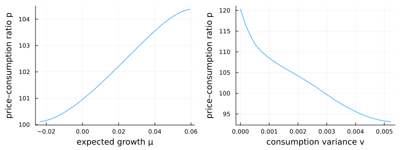

This page was generated using Literate.jl.