Tuckman–Vila (1992): a finite-horizon problem

So far every model has been stationary. Tuckman–Vila is time-dependent: an arbitrageur faces holding costs over a finite horizon $[0, T]$, so the value function $F(z, \tau)$ depends on calendar time. pdesolve handles this by taking a time grid τs as a fourth argument and solving backward from a terminal condition. The PDE function then takes a third argument τ:

\[\partial_\tau F + \max_i\Bigl\{ (\mu + \sigma^2 F_z)\, a i - \tfrac12 \sigma^2 (a i)^2 \Bigr\} - \rho z F_z + \tfrac12 \sigma^2 (F_{zz} - F_z^2) = 0.\]

Defining the model

The parameters live in a struct:

using EconPDEs, Distributions, Plots

Base.@kwdef struct TuckmanVilaModel
    c::Float64 = 0.06     # coupon rate of the bond
    r::Float64 = 0.09     # risk-free rate
    ρ::Float64 = 5.42     # mean-reversion speed of the state z
    σ::Float64 = 26.72    # volatility of the state z
    a::Float64 = 26.72    # position (holding-cost) scaling parameter
    T::Float64 = 100      # horizon (terminal date)
end

Main.TuckmanVilaModel

We solve the model at its default parameters:

m = TuckmanVilaModel()

Main.TuckmanVilaModel(0.06, 0.09, 5.42, 26.72, 26.72, 100.0)

Defining the grid

We define the grid, a NamedTuple whose key is the state variable (z). The grid spans the stationary range of $z$ (a mean-reverting Gaussian). Because the problem is finite-horizon, we also build a time grid τs over $[0, T]$, which pdesolve will march backward along.

function initialize_stategrid(m::TuckmanVilaModel; zn = 200)
    d = Normal(0, sqrt(m.σ^2 / (2 * m.ρ)))
    (; z = range(quantile(d, 0.00001), quantile(d, 0.99999), length = zn))
end

initialize_stategrid (generic function with 1 method)

Defining an initial guess

We define the initial guess, a NamedTuple whose key is the unknown function (F), which here doubles as the terminal condition at τs[end]. These names (and the finite differences of $F$, such as Fz_up) are what reappear in the equation below. We then build the grid, guess, and time grid from the model:

function initialize_guess(m::TuckmanVilaModel, stategrid)
    zn = length(stategrid[:z])
    (; F = zeros(zn))
end

stategrid = initialize_stategrid(m)
guess = initialize_guess(m, stategrid)
τs = range(0, m.T, length = 10)

0.0:11.11111111111111:100.0

Defining the PDE

We now write the function encoding the HJB equation. Following the package convention, it takes the current state (a grid point) and u (each unknown together with its finite-difference derivatives there) and returns the time derivative of each unknown. Because the problem is time-dependent, it also takes a third argument, the time τ.

function (m::TuckmanVilaModel)(state::NamedTuple, u::NamedTuple, τ::Number)
    (; c, r, ρ, σ, a, T) = m
    (; z) = state
    (; F, Fz_up, Fz_down, Fzz) = u
    Fz = (z >= 0) ? Fz_up : Fz_down
    ϕ = z * (1 + z^2)^(-1 / 2)
    ϕz = (1 + z^2)^(-3 / 2)
    ϕzz = -3 * z * (1 + z^2)^(-5 / 2)
    sτ = c / r * (1 - exp(-r * (T - τ)))
    μL = ρ * z - 0.5 * σ^2 * ϕzz / ϕz + c / sτ * (ϕ - 1) / ϕz
    iL = 1 / a * (μL / σ^2 + Fz)
    μS = ρ * z - 0.5 * σ^2 * ϕzz / ϕz + c / sτ * (ϕ + 1) / ϕz
    iS = 1 / a * (μS / σ^2 + Fz)
    μ, i = 0.0, 0.0
    if iL > 0
        i, μ = iL, μL
    elseif iS < 0
        i, μ = iS, μS
    end
    Ft = -((μ + σ^2 * Fz) * a * i - 0.5 * σ^2 * (a * i)^2 - ρ * z * Fz + 0.5 * σ^2 * (Fzz - Fz^2))
    return (; Ft)
end

Solving the model

pdesolve takes the time grid τs as a fourth argument and marches backward from the terminal condition:

result = pdesolve(m, stategrid, guess, τs)

EconPDEResult (time-dependent, 10 times; last dimension is time)
  solution:      F (200×10)
  residual_norm: 2.08e-10 (max over times)
  converged:     true (tolerance 1.49e-08)

The solution

For a time-dependent problem each solution array has a trailing time dimension: result.solution.F[:, i] is the solution at time τs[i] (so result.solution.F[:, end] is the terminal condition). To make the backward time dimension visible, we fix a representative state near $z = 0$ and plot its value over calendar time. The value falls to the terminal condition $F = 0$ as $\tau$ approaches $T$.

zs = stategrid[:z]
z0_index = argmin(abs.(zs))
F_at_z0 = result.solution.F[z0_index, :]
plot(τs, F_at_z0; xlabel = "time τ", ylabel = "value F(z ≈ 0, τ)", legend = false)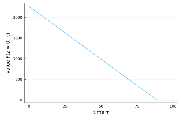

This page was generated using Literate.jl.