Gomez (2025): wealth inequality and asset prices
An asset-pricing model with a wealth-distribution state. Households and entrepreneurs differ in preferences and in the risk they bear; entrepreneurs hold a leveraged position in the risky asset, so shifts in the wealth distribution move the price of risk and the volatility of returns. The single state $x$ is the entrepreneurs' consumption share, and the unknown is the households' wealth–consumption ratio $p_H$. Demographics (birth, death, and entry of entrepreneurs) keep the distribution stationary.
Defining the model
The parameters:
using EconPDEs, Plots

Base.@kwdef struct GomezModel
    # utility, households
    γ::Float64 = 10.3      # households' relative risk aversion
    ψ::Float64 = 0.05      # households' elasticity of intertemporal substitution
    ρ::Float64 = 0.1       # households' discount rate

    # utility, entrepreneurs
    ρE::Float64 = 0.022    # entrepreneurs' discount rate
    αE::Float64 = 2        # entrepreneurs' risk aversion
    ν::Float64 = 0.1       # entrepreneurs' preference parameter

    # demography
    η::Float64 = 0.015     # birth rate
    δ::Float64 = 0.025     # death rate
    ϕ::Float64 = 0.01      # demographic transition rate
    πE::Float64 = 0.09     # entry rate into entrepreneurship

    # endowment process
    g::Float64 = 0.02      # expected consumption growth
    σ::Float64 = 0.04      # consumption volatility
    λ::Float64 = 2.3       # endowment-process parameter
    τ::Float64 = 0.0       # tax rate
endMain.GomezModelWe solve the model at its default parameters:
m = GomezModel()Main.GomezModel(10.3, 0.05, 0.1, 0.022, 2.0, 0.1, 0.015, 0.025, 0.01, 0.09, 0.02, 0.04, 2.3, 0.0)Defining the grid
We define the grid, a NamedTuple keyed by the state variable $x$, the entrepreneurs' consumption share. It spans $[0, 1]$ but is squared, concentrating points near $x = 0$ where entrepreneurs are scarce and the wealth-distribution dynamics are sharpest.
stategrid = (; x = range(0, 1, 300) .^ 2)(x = [0.0, 1.1185557208532343e-5, 4.474222883412937e-5, 0.0001006700148767911, 0.0001789689153365175, 0.00027963893021330853, 0.0004026800595071644, 0.0005480923032180848, 0.00071587566134607, 0.0009060301338911198 … 0.9407053612375701, 0.9472041699757274, 0.9537253498283017, 0.9602689007952931, 0.9668348228767016, 0.9734231160725272, 0.9800337803827698, 0.9866668158074294, 0.9933222223465062, 1.0],)Defining an initial guess
We define the initial guess, a NamedTuple whose key is the single unknown function (pH, the households' wealth–consumption ratio), initialized flat at one. This name — and its finite differences, such as pHx_up — is what reappears inside the equation below.
guess = (; pH = ones(length(stategrid[:x])))(pH = [1.0, 1.0, 1.0, 1.0, 1.0, 1.0, 1.0, 1.0, 1.0, 1.0 … 1.0, 1.0, 1.0, 1.0, 1.0, 1.0, 1.0, 1.0, 1.0, 1.0],)Defining the PDE
We now write the function encoding the equilibrium conditions. Following the package convention, it takes the current state (a grid point) and u — the local bundle holding the unknown and its finite-difference derivatives there — and returns the time derivative of the unknown (pHt).
The volatility of the state $\sigma_x$ is endogenous, feeding back through prices, so the upwind direction is picked from the drift $\mu_x$: forward difference pHx_up unless the drift turns negative, then backward pHx_down.
function (m::GomezModel)(state::NamedTuple, u::NamedTuple)
  (; γ, ψ, ρ, ρE, αE, ν, η, δ, ϕ, πE, g, σ, λ, τ) = m
  (; x) = state
  (; pH, pHx_up, pHx_down, pHxx) = u
  p = x / ρE + (1 - x) * pH
  xW = x / ρE / p
  # Effective entrepreneur exposure, capped when the leverage constraint xW * αE ≥ 1 binds.
  αEeff = (xW * αE >= 1) ? 1 / xW : αE
  iter = 0
  pHx = pHx_up
  @label start
  px = 1 / ρE  - pH + (1 - x) * pHx
  σx = x * (αEeff - 1) * σ / (1 - x * αEeff * px / p)
  σpH = pHx / pH * σx
  σp = px / p * σx
  σCE = αEeff * (σ + σp)
  σCH = x < 1 ? (σ - x * σCE) / (1 - x) : 0.0
  σWH = σCH + σpH
  κ = γ * σCH + (γ * ψ - 1) / (ψ - 1) * σpH
  ΦE = αEeff * κ * (σ + σp)
  ΦH = κ^2 * (1 + ψ) / (2 * γ) + (1 - ψ * γ) / (γ * (ψ - 1)) * κ * σpH - (1 - γ * ψ) / (2 * γ * (ψ - 1)) * σpH^2
  arriving_wealth = (η + δ + ϕ + τ) / (η + δ) * p
  wedge = (η + δ) * ((ρE * πE + (1 - πE) / pH) * arriving_wealth - 1)
  Ψ = x + (1 - x) * ψ
  P = (x * ρE + (1 - x) * ψ * ρ) / Ψ
  r = P + 1 / Ψ * (g - x * ΦE - (1 - x) * ΦH - wedge) + τ
  μCE = r - τ -  ρE + ΦE
  μCH = ψ * (r - τ - ρ) + ΦH
  μx = x * (μCE - g) + (η + δ) * (ρE * πE * arriving_wealth - x) - σ * σx
  if (iter == 0) & (μx <= 0)
    iter += 1
    pHx = pHx_down
    @goto start
  end
  μpH = pHx / pH * μx + 0.5 * pHxx / pH * σx^2
  pxx = - 2 * pHx + (1 - x) * pHxx
  μp = px / p * μx + 0.5 * pxx / p * σx^2
  μWH = μCH + μpH + σCH * σpH
  pHt = - pH * (1 / pH + μWH - r + τ - κ * σWH)
  σR = σ + σp
  μR = r + κ * σR
  σWE = σCE
  σErelative = (αEeff - 1) * (σ + σp)
  μErelative = μCE - (g + μp + σ * σp) - σErelative * (σ + σp)
  α = x < 1 ? (1 - xW * αEeff) / (1 - xW) : 0.0
  σHrelative = (α - 1) * (σ + σp)
  μHrelative = μWH - (g + μp + σ * σp) - σHrelative * (σ + σp)
  μxW = xW * (μCE - (g + μp + σ * σp) - σErelative * (σ + σp)) + (η + δ) * (πE * (η + δ + ϕ) / (η + δ) - xW)
  σxW = xW * (αEeff - 1) * (σ + σp)
  μRλ = r + λ * (μR - r)
  σRλ = λ * σR
  return (; pHt), (; x, μx, σx, κ, r, σWH, μWH, σp, p, px, σR, μR, μRλ, σRλ, μErelative, σErelative, μHrelative, σHrelative, μCE, μxW, σxW, pH, μCH, wedge, xW, σWE, σCH, αE = αEeff, pE = 1 / m.ρE, μp = μp)
end
Solving the model
With the grid, guess, and equation in hand, pdesolve solves the stationary system:
result = pdesolve(m, stategrid, guess)EconPDEResult
solution: pH (300)
saved: pH, x, μx, σx, κ, r, σWH, μWH, σp, p, px, σR, μR, μRλ, σRλ, μErelative, σErelative, μHrelative, σHrelative, μCE, μxW, σxW, μCH, wedge, xW, σWE, σCH, αE, pE, μp
residual_norm: 1.06e-10
converged: true (tolerance 1.49e-08)The solution
We saved the volatility of the risky return $\sigma_R$. It differs from the fundamental volatility $\sigma$ because prices themselves move with the wealth distribution — endogenous amplification — and the size of that wedge varies with the entrepreneurs' consumption share $x$.
xs = stategrid[:x]
plot(xs, result.saved.σR; xlabel = "entrepreneurs' consumption share x", ylabel = "return volatility σR", legend = false)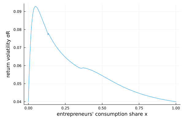
This page was generated using Literate.jl.