Wang–Wang–Yang (2016): consumption and saving with recursive utility

Wang, Wang, and Yang (2016) study optimal consumption and saving when labor income follows a geometric Brownian motion, $dY = \mu Y\,dt + \sigma Y\,dZ$, and the household has recursive (Epstein–Zin) preferences with elasticity of intertemporal substitution $\psi$ and risk aversion $\gamma$. Wealth accumulates as $dX = (r X + Y - C)\,dt$ subject to a borrowing limit. Because income is a GBM and preferences are homothetic, the value function is homogeneous and the problem collapses to a single ODE in the wealth-to-income ratio $w = X/Y$. Writing $p(w)$ for the scaled value function — equivalently, total wealth (financial plus human) per unit of income — it solves

\[0 = \left(\frac{(r + \psi(\rho - r))\,p'^{\,1-\psi} - \psi\rho}{\psi - 1} + \mu - \tfrac{\gamma\sigma^2}{2}\right) p + \bigl((r - \mu + \gamma\sigma^2)\,w + 1\bigr)\, p' + \tfrac12 \sigma^2 w^2\left(p'' - \gamma\,\frac{p'^{\,2}}{p}\right),\]

with the consumption–income ratio recovered from $c = (r + \psi(\rho - r))\, p\, p'^{-\psi}$.

Defining the model

The parameters live in a struct:

using EconPDEs, Plots, Printf

Base.@kwdef struct WangWangYangModel
    μ::Float64 = 0.015       # expected growth rate of labor income
    σ::Float64 = 0.1         # volatility of labor income
    r::Float64 = 0.035       # risk-free rate
    ρ::Float64 = 0.04        # discount rate
    γ::Float64 = 3.0         # relative risk aversion
    ψ::Float64 = 1.1         # elasticity of intertemporal substitution
    wmin::Float64 = 0.0      # borrowing limit (minimum wealth-income ratio)
    wmax::Float64 = 1000.0   # maximum wealth-income ratio (grid upper bound)
end

Main.WangWangYangModel

We solve the model at its default parameters:

m = WangWangYangModel()

Main.WangWangYangModel(0.015, 0.1, 0.035, 0.04, 3.0, 1.1, 0.0, 1000.0)

Defining the grid

We define the grid, a NamedTuple keyed by the state $w$ (the wealth-to-income ratio), running from the borrowing limit to a large upper bound on a simple linear grid.

stategrid = (; w = range(m.wmin, m.wmax, length = 1001))

(w = 0.0:1.0:1000.0,)

Defining an initial guess

We define the initial guess, a NamedTuple keyed by the unknown function $p$ — one value per grid point. The guess $p = 1 + w$ reflects total wealth as financial plus one unit of human wealth. This name (and its finite differences, such as pw_up) is what reappears in the equation below.

guess = (; p = 1 .+ stategrid[:w])

(p = 1.0:1.0:1001.0,)

Defining the PDE

We now write the function encoding the HJB equation. Following the package convention, it takes the current state (a grid point) and u (each unknown together with its finite-difference derivatives there) and returns the time derivative of each unknown.

We upwind on the physical wealth drift $\mu_w$ of the controlled state, falling back to $\mu_w = 0$ when the borrowing constraint binds.

function (m::WangWangYangModel)(state::NamedTuple, u::NamedTuple)
    (; μ, σ, r, ρ, γ, ψ, wmin, wmax) = m
    (; w) = state
    (; p, pw_up, pw_down, pww) = u
    mstar = r + ψ * (ρ - r)
    p_for_trial = max(p, eps())
    # Newton can try negative marginal values, so cap implied consumption instead of flooring derivatives.
    cmax = 100.0 * (1 + max((r - μ + σ^2) * w, 0.0))

    # Upwind on the physical wealth drift of the controlled state process.
    c_up = pw_up > 0 ? min(mstar * p * pw_up^(-ψ), cmax) : cmax
    μw_up = (r - μ + σ^2) * w + 1 - c_up
    if μw_up >= 0
        # Keep the branch condition about upwinding. If a Newton trial made the selected
        # marginal value nonpositive, use the marginal value implied by capped consumption
        # only to keep the residual's fractional power well-defined.
        pw = pw_up > 0 ? pw_up : (c_up / (mstar * p_for_trial))^(-1 / ψ)
        c = c_up
        μw = μw_up
    else
        c_down = pw_down > 0 ? min(mstar * p * pw_down^(-ψ), cmax) : cmax
        μw_down = (r - μ + σ^2) * w + 1 - c_down
        if (μw_down <= 0) && (w > wmin)
            pw = pw_down > 0 ? pw_down : (c_down / (mstar * p_for_trial))^(-1 / ψ)
            c = c_down
            μw = μw_down
        else
            # If the two candidates straddle zero OR drift is negative at minimum asset threshold
            # we impose drift μw = 0.
            μw = 0.0
            c = 1 + (r - μ + σ^2) * w
            pw = (c / (mstar * p_for_trial))^(-1 / ψ)
        end
    end
    # At the top, we use the solution of the unconstrained problem, i.e. pw = 1 (a reflecting boundary would also work but is less elegant).
    pt = - ((((r + ψ * (ρ - r)) * pw^(1 - ψ) - ψ * ρ) / (ψ - 1) + μ - γ * σ^2 / 2) * p + ((r - μ + γ * σ^2) * w + 1) * pw + σ^2 * w^2 / 2  * (pww - γ * pw^2 / p))
    return (; pt), (; c, μw)
end

Solving the model

With the grid, guess, and equation in hand, pdesolve solves the stationary system. The bc entry supplies one-sided ghost derivatives at the edges of the grid. At the borrowing constraint, the PDE still uses the inward derivative when the drift points into the state space, so the economically relevant $p'(0)$ is determined by the solution; at the upper edge, the condition pins the asymptotic complete-markets marginal value $p'(w) \to 1$.

result = pdesolve(m, stategrid, guess, bc = (; pw = (1.0, 1.0)))

EconPDEResult
  solution:      p (1001)
  saved:         p, c, μw
  residual_norm: 7.62e-10
  converged:     true (tolerance 1.49e-08)

The solution

The paper reports the baseline solution on $w \in [0,20]$. We use a wider $w \in [0,100]$ window for the level and consumption panels, because it makes the convergence toward the complete-markets benchmark visible while still showing the low-wealth wedge. The derivative panel stays on $w \in [0,20]$, where the liquidity-premium curvature is concentrated. We compute finite-difference slopes for $p'(w)$ and compare the solution with the complete-markets benchmarks $p^*(w) = w + h$ and $c^*(w) = m^* (w + h)$.

ws = stategrid[:w]
p = result.solution.p
c = result.saved.c
h = 1 / (m.r - m.μ)
mstar = m.r + m.ψ * (m.ρ - m.r)
wmid = (ws[1:(end - 1)] .+ ws[2:end]) ./ 2
pprime = diff(p) ./ diff(ws)

p0 = p[1]
pprime0 = pprime[1]
@printf("p(0) = %.2f, versus complete-markets p*(0) = %.2f; p(0)/p*(0) = %.1f%%\n",
        p0, h, 100 * p0 / h)
@printf("p'(0) = %.2f, so one dollar of liquid wealth is worth %.1f%% more than its accounting value at the constraint\n",
        pprime0, 100 * (pprime0 - 1))

wideidx = ws .<= 100
didx = wmid .<= 20
p1 = plot(ws[wideidx], p[wideidx]; xlabel = "wealth-income ratio w", ylabel = "p(w)",
          label = "model", xlims = (0, 100), ylims = (20, 160))
plot!(p1, ws[wideidx], ws[wideidx] .+ h; label = "complete markets", linestyle = :dash)
p2 = plot(wmid[didx], pprime[didx]; xlabel = "wealth-income ratio w", ylabel = "p'(w)",
          label = "model", xlims = (0, 20), ylims = (1.0, 1.5))
hline!(p2, [1.0]; label = "complete markets", linestyle = :dash)
p3 = plot(ws[wideidx], c[wideidx]; xlabel = "wealth-income ratio w", ylabel = "c(w)",
          label = "model", xlims = (0, 100), ylims = (0.5, 6.5))
plot!(p3, ws[wideidx], mstar .* (ws[wideidx] .+ h); label = "complete markets", linestyle = :dash)
plot(p1, p2, p3; layout = (1, 3), size = (900, 420),
     left_margin = 5Plots.mm, bottom_margin = 8Plots.mm)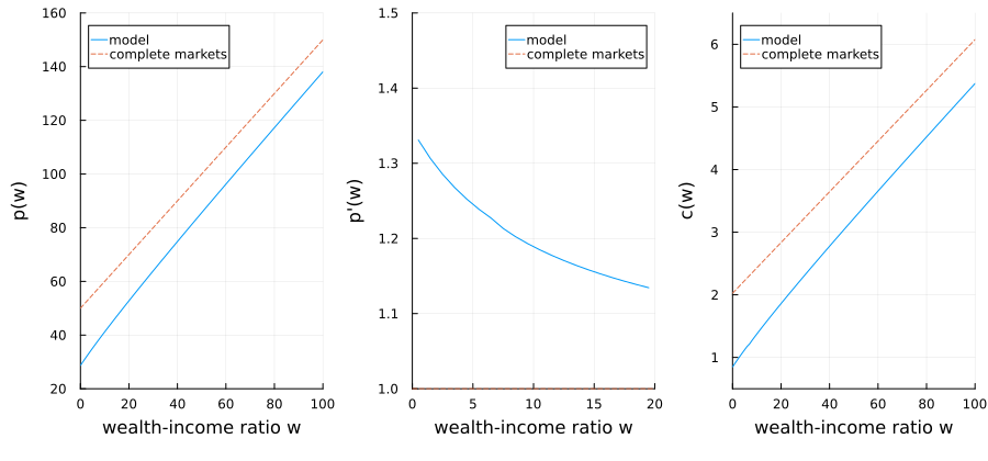

The level $p(0)$ is the certainty-equivalent value, in units of current income, of an agent who has no liquid wealth but still receives stochastic labor income. The gap between $p(0)$ and $p^*(0) = h$ is the welfare cost of incomplete markets and the borrowing constraint. The slope $p'(0)$ is the marginal certainty-equivalent value of one more dollar of liquid wealth at the constraint; values above one are a liquidity premium. As wealth rises, self-insurance becomes more effective, so $p'(w)$ falls toward the complete-markets value one and $p(w)$ approaches the linear benchmark $w + h$.

This page was generated using Literate.jl.