Leland (1994): optimal default

Leland's model of a levered firm is a classic optimal-stopping problem. The full paper values risky debt and studies capital structure; this example isolates the equityholders' default decision. Cash flow (EBIT) $\delta$ follows a geometric Brownian motion $d\delta = \mu\delta\,dt + \sigma\delta\,dW$. The firm has issued perpetual debt with coupon $C$ and faces a tax rate $\tau$; equity holders receive the after-tax flow $\delta-(1-\tau)C$ but may default (walk away) whenever they choose. Equity value $E(\delta)$ is thus the value of the option to keep the firm alive, and solves the HJB variational inequality

\[\min\Bigl\{\, r E - \bigl(\delta-(1-\tau)C\bigr) - \mu\delta\,E'(\delta) - \tfrac12\sigma^2\delta^2 E''(\delta),\;\; E(\delta)\,\Bigr\} = 0,\]

with default payoff $0$ (limited liability). This delivers the value-matching $E(\delta^*)=0$ and smooth-pasting $E'(\delta^*)=0$ conditions at the endogenous default threshold $\delta^*$.

Defining the model

The parameters live in a struct:

using EconPDEs, Plots, Printf

Base.@kwdef struct LelandModel
    r::Float64 = 0.02    # risk-free rate
    μ::Float64 = 0.0     # drift of cash flow (EBIT growth)
    σ::Float64 = 0.1     # volatility of cash flow
    C::Float64 = 0.05    # coupon rate
    τ::Float64 = 0.2     # tax rate
end

Main.LelandModel

We solve the model at its default parameters:

m = LelandModel()

Main.LelandModel(0.02, 0.0, 0.1, 0.05, 0.2)

Defining the grid

We define the grid, a NamedTuple keyed by the state $δ$ (the cash flow).

stategrid = (; δ = range(0, 0.2, step = 0.005))

(δ = 0.0:0.005:0.2,)

Defining an initial guess

We define the initial guess, a NamedTuple keyed by the unknown function $E$ (equity value) — one value per grid point, the value of the cash-flow claim net of the after-tax coupon, floored at zero. This name (and its finite differences, such as Eδ_up) is what reappears in the equation below.

guess = (; E = max.(stategrid[:δ] ./ (m.r - m.μ) .- (1 .- m.τ) .* m.C ./ m.r, 0.0))

(E = [0.0, 0.0, 0.0, 0.0, 0.0, 0.0, 0.0, 0.0, 0.0, 0.24999999999999956  …  5.75, 6.0, 6.25, 6.5, 6.75, 7.0, 7.25, 7.5, 7.75, 8.0],)

Defining the PDE

We now write the function encoding the HJB equation. Following the package convention, it takes the current state (a grid point) and u (each unknown together with its finite-difference derivatives there) and returns the time derivative of each unknown.

function (m::LelandModel)(state::NamedTuple, u::NamedTuple)
    (; r, μ, σ, C, τ) = m
    (; δ) = state
    (; E, Eδ_up, Eδ_down, Eδδ) = u
    μδ, σδ = μ * δ, σ * δ
    Eδ = (μδ >= 0) ? Eδ_up : Eδ_down
    f = δ - (1 - τ) * C
    Et = -(f + Eδ * μδ + 0.5 * Eδδ * σδ^2 - r * E)
    return (; Et)
end

Solving the model

The stopping (default) region is imposed by passing zero as lower_bound: equity can never be worth less than zero. We also pin the slope at the top boundary to that of a debt-free claim, $1/(r-\mu)$. With these in hand, pdesolve solves the variational inequality:

lower_bound = zeros(length(stategrid[:δ]))
bc = (; Eδ = (0.0, 1 / (m.r - m.μ)))
result = pdesolve(m, stategrid, guess; lower_bound = lower_bound, bc = bc)

EconPDEResult
  solution:      E (41)
  residual_norm: 2.06e-11
  converged:     true (tolerance 1.49e-08)

The solution

Equity is worthless below an endogenous default threshold $\delta^*$ and rises smoothly above it. This stripped-down case has the familiar closed-form trigger. If $\beta < 0$ is the negative root of

\[\tfrac12\sigma^2\beta(\beta-1) + \mu\beta - r = 0,\]

then

\[\delta^* = \frac{\beta}{\beta-1}\,(r-\mu)\,\frac{(1-\tau)C}{r}.\]

The finite-difference solution recovers the same boundary up to grid resolution. In the plot, the red dotted line is the closed-form trigger and the gray dashed line is the first grid point where the variational-inequality solution lifts off from zero.

δs = stategrid[:δ]
E = result.solution.E
# Default boundary δ*: the first grid point where equity lifts off the E = 0 lower bound of the variational inequality.
δstar_grid = δs[findfirst(>(1e-8), E)]
root_a = 0.5 * m.σ^2
root_b = m.μ - 0.5 * m.σ^2
root_c = -m.r
β = min((-root_b + sqrt(root_b^2 - 4 * root_a * root_c)) / (2 * root_a),
        (-root_b - sqrt(root_b^2 - 4 * root_a * root_c)) / (2 * root_a))
δstar = β / (β - 1) * (m.r - m.μ) * (1 - m.τ) * m.C / m.r
claim_slope = 1 / (m.r - m.μ)
coupon_value = (1 - m.τ) * m.C / m.r
option_loading = -claim_slope * δstar^(1 - β) / β
continuation = δs .>= δstar_grid
E_closed = zeros(length(δs))
E_closed[continuation] .= claim_slope .* δs[continuation] .- coupon_value .+
                          option_loading .* δs[continuation].^β
@printf("closed-form default threshold δ* = %.4f; grid lift-off = %.4f\n",
        δstar, δstar_grid)
@printf("maximum equity-value error on the continuation grid = %.2e\n",
        maximum(abs.(E[continuation] .- E_closed[continuation])))
plot(δs, E; xlabel = "cash flow δ", ylabel = "equity value E(δ)",
     label = "finite difference", legend = :topleft)
plot!(δs[continuation], E_closed[continuation]; color = :black, linestyle = :dash,
      label = "closed form")
vline!([δstar]; color = :red, linestyle = :dot, label = "closed-form δ*")
vline!([δstar_grid]; color = :gray, linestyle = :dash, label = "grid lift-off")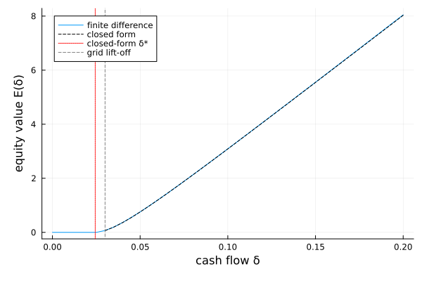

This page was generated using Literate.jl.