Achdou–Han–Lasry–Lions–Moll: consumption–saving with two income states

A household saves in a riskless asset $a$ at rate $r$ and earns a labor income that switches between a low value $y_l$ and a high value $y_h$ as a two-state Poisson process (intensities $\lambda_{lh}$, $\lambda_{hl}$). There is one continuous state (assets $a$) but two coupled value functions $v_l(a)$ and $v_h(a)$, one per income state, linked by the income transitions:

\[\rho\, v_j(a) = \max_c \frac{c^{1-\gamma}}{1-\gamma} + v_j'(a)\,(y_j + r a - c) + \lambda_{jk}\,\bigl(v_k(a)-v_j(a)\bigr), \qquad j \ne k.\]

A borrowing constraint $a \ge \underline a$ is enforced by preventing the asset drift from turning negative at the lower bound.

The model

The parameters live in a struct:

using EconPDEs, Plots

Base.@kwdef mutable struct AchdouHanLasryLionsMollModel_TwoStates
    yl::Float64 = 0.5        # low income state
    yh::Float64 = 1.5        # high income state
    λlh::Float64 = 0.2       # low → high transition intensity
    λhl::Float64 = 0.2       # high → low transition intensity
    r::Float64 = 0.03        # risk-free rate
    ρ::Float64 = 0.04        # discount rate
    γ::Float64 = 2.0         # relative risk aversion
    amin::Float64 = -yl / r  # borrowing limit (natural limit)
    amax::Float64 = 50.0     # top of the asset grid
end

Main.AchdouHanLasryLionsMollModel_TwoStates

We solve the model at its default parameters:

m = AchdouHanLasryLionsMollModel_TwoStates()

Main.AchdouHanLasryLionsMollModel_TwoStates(0.5, 1.5, 0.2, 0.2, 0.03, 0.04, 2.0, -16.666666666666668, 50.0)

The grid

We define the grid, a NamedTuple keyed by the single continuous state $a$. The asset grid is finer near the borrowing limit, where consumption is most curved; the borrowing limit itself is nudged just inside the natural limit $-y_l/r$ to keep consumption strictly positive there.

m.amin += 0.001
stategrid = (; a = m.amin .+ range(0, (m.amax - m.amin)^(1 / 2), length = 200) .^ 2)

(a = [-16.665666666666667, -16.66398323274665, -16.65893293098659, -16.650515761386497, -16.638731723946364, -16.623580818666195, -16.60506304554599, -16.58317840458574, -16.55792689578546, -16.52930851914514  …  44.10629784601399, 44.747686169541176, 45.3924413609084, 46.040563420115646, 46.69205234716295, 47.34690814205027, 48.00513080477765, 48.66672033534506, 49.331676733752516, 50.0],)

The initial guess

We define the initial guess, a NamedTuple keyed by the two unknown value functions $v_l$ and $v_h$ — one autarky-style starting value per grid point. These names (and their finite differences, such as vla_up) are what reappear in the equation below.

guess = (;
    vl = (m.ρ ./ m.γ .+ (1 .- 1 / m.γ) .* m.r)^(-m.γ) .* (stategrid[:a] .+ m.yl ./ m.r) .^ (1 - m.γ) ./ (1 - m.γ),
    vh = (m.ρ ./ m.γ .+ (1 .- m.γ) .* m.r)^(-m.γ) .* (stategrid[:a] .+ m.yh ./ m.r) .^ (1 - m.γ) ./ (1 - m.γ),
)

(vl = [-816326.5306112472, -304209.66379019007, -105553.97344587464, -50543.70120135009, -29222.416483385914, -18946.51187098101, -13251.275099772196, -9777.740130953549, -7507.156985865249, -5943.051397692311  …  -13.432396085300613, -13.29211320991021, -13.154016494235172, -13.018060748058993, -12.884201942814869, -12.752397175935922, -12.622604636475304, -12.49478357194475, -12.3688942563225, -12.244897959183671], vh = [-299.991000269992, -299.9758510387842, -299.93041252401383, -299.8547122483401, -299.7487960365673, -299.61272794634107, -299.44659017139617, -299.25048291762994, -299.0245242523482, -298.7688499271064  …  -106.26281374242339, -105.543474508771, -104.8301087312142, -104.12267112861927, -103.42111639223482, -102.72539920228213, -102.03547424389043, -101.35129622239745, -100.67281987803234, -100.00000000000004])

The PDE equation

We now write the function encoding the HJB equation. Following the package convention, it takes the current state (a grid point) and u (each unknown together with its finite-difference derivatives there) and returns the time derivative of each unknown.

In each income state we upwind the asset drift on its sign, capping the implied consumption rather than flooring the marginal value (Newton may try negative marginal values). At the borrowing constraint the drift is set to zero. We save consumption cl, ch to plot.

function (m::AchdouHanLasryLionsMollModel_TwoStates)(state::NamedTuple, u::NamedTuple)
    (; yl, yh, λlh, λhl, r, ρ, γ, amin, amax) = m
    (; a) = state
    (; vl, vla_up, vla_down, vh, vha_up, vha_down) = u
    clmax = 100.0 * (yl + r * max(a, 0.0))
    chmax = 100.0 * (yh + r * max(a, 0.0))

    # upwind the low-income value function
    cl_up = vla_up > 0 ? min(vla_up^(-1 / γ), clmax) : clmax
    μla_up = yl + r * a - cl_up
    if μla_up >= 0.0
        vla, cl, μla = vla_up, cl_up, μla_up
    else
        cl_down = vla_down > 0 ? min(vla_down^(-1 / γ), clmax) : clmax
        μla_down = yl + r * a - cl_down
        if μla_down <= 0.0 && a > amin
            vla, cl, μla = vla_down, cl_down, μla_down
        else
            cl = yl + r * a          # borrowing constraint binds: drift is zero
            μla = 0.0
            vla = cl^(-γ)
        end
    end
    vlt = -(cl^(1 - γ) / (1 - γ) + μla * vla + λlh * (vh - vl) - ρ * vl)

    # upwind the high-income value function
    ch_up = vha_up > 0 ? min(vha_up^(-1 / γ), chmax) : chmax
    μha_up = yh + r * a - ch_up
    if μha_up >= 0.0
        vha, ch, μha = vha_up, ch_up, μha_up
    else
        ch_down = vha_down > 0 ? min(vha_down^(-1 / γ), chmax) : chmax
        μha_down = yh + r * a - ch_down
        if μha_down <= 0.0 && a > amin
            vha, ch, μha = vha_down, ch_down, μha_down
        else
            ch = yh + r * a
            μha = 0.0
            vha = ch^(-γ)
        end
    end
    vht = -(ch^(1 - γ) / (1 - γ) + μha * vha + λhl * (vl - vh) - ρ * vh)

    return (; vlt, vht), (; cl, ch, μla, μha)
end

Solving the model

With the grid, guess, and equation in hand, pdesolve solves the stationary system:

result = pdesolve(m, stategrid, guess)

EconPDEResult
  solution:      vl (200), vh (200)
  saved:         vl, vh, cl, ch, μla, μha
  residual_norm: 3.13e-11
  converged:     true (tolerance 1.49e-08)

The solution

Consumption rises with wealth in both income states and is higher when income is high (left). The saving rate (right) is pinned at zero at the borrowing limit for the low-income household — which is forced to consume its income $y_l + r a$ — and turns positive as wealth rises.

as = stategrid[:a]
idx = 1:div(length(as), 3)          # left third of the asset grid, where the curvature is
p1 = plot(as[idx], [result.saved.cl[idx] result.saved.ch[idx]]; label = ["low income" "high income"], xlabel = "assets a", ylabel = "consumption c(a)", legend = :bottomright)
p2 = plot(as[idx], [result.saved.μla[idx] result.saved.μha[idx]]; label = ["low income" "high income"], xlabel = "assets a", ylabel = "saving μa(a)", legend = :topright)
hline!(p2, [0.0]; color = :gray, linestyle = :dash, label = "")
plot(p1, p2; layout = (1, 2), size = (800, 300))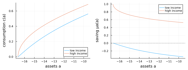

This page was generated using Literate.jl.