Achdou–Han–Lasry–Lions–Moll: consumption–saving with diffusion income

This is the diffusive-income version of the Achdou–Han–Lasry–Lions–Moll (2022) consumption– saving problem, the standard building block of continuous-time heterogeneous-agent (HACT) models. A household earns stochastic labor income $y$, saves in a single riskless asset $a$ at rate $r$, and cannot borrow past a limit $a \ge a_{\min}$. Income mean-reverts as a diffusion, and the value function $v(y, a)$ solves the Hamilton–Jacobi–Bellman equation

\[\rho\, v = \max_{c}\; \frac{c^{1-\gamma}}{1-\gamma} + \partial_a v\,\bigl(y + r a - c\bigr) + \partial_y v\,\kappa_y(\bar y - y) + \tfrac12 \sigma_y^2\, \partial_{yy} v,\]

with first-order condition $c = (\partial_a v)^{-1/\gamma}$ and the borrowing constraint $a \ge a_{\min}$ enforced as a state constraint (saving cannot be negative at the limit).

The model

The parameters live in a struct:

using EconPDEs, Distributions, Plots

Base.@kwdef struct AchdouHanLasryLionsMollModel_Diffusion
    κy::Float64 = 0.1      # income mean-reversion speed
    ybar::Float64 = 1.0    # mean income level
    σy::Float64 = 0.07     # income volatility
    r::Float64 = 0.03      # risk-free rate
    ρ::Float64 = 0.05      # discount rate
    γ::Float64 = 2.0       # relative risk aversion
    amin::Float64 = 0.0    # borrowing limit
    amax::Float64 = 100.0  # top of the asset grid
end

Main.AchdouHanLasryLionsMollModel_Diffusion

We solve the model at its default parameters:

m = AchdouHanLasryLionsMollModel_Diffusion()

Main.AchdouHanLasryLionsMollModel_Diffusion(0.1, 1.0, 0.07, 0.03, 0.05, 2.0, 0.0, 100.0)

The grid

We define the grid, a NamedTuple keyed by the state variables $y$ and $a$. Income spans the bulk of its ergodic (Gamma) distribution; assets run from the borrowing limit $a_{\min}$ up to $a_{\max}$.

distribution = Gamma(2 * m.κy * m.ybar / m.σy^2, m.σy^2 / (2 * m.κy))
stategrid = (; y = range(quantile(distribution, 0.001), quantile(distribution, 0.999), length = 10),
                        a =  range(m.amin, m.amax, length = 1000)
                        )

(y = 0.5850212023872049:0.10767961021653895:1.5541376943360554, a = 0.0:0.1001001001001001:100.0)

The initial guess

We define the initial guess, a NamedTuple keyed by the unknown $v$ — one value per grid point, here the value of consuming the annuity value of total wealth $a + y/r$ forever. These names (and the finite differences of $v$, such as va_up) are what reappear in the equation below.

guess = (; v = [(m.ρ / m.γ + (1 - 1 / m.γ) * m.r)^(-m.γ) * (a + y / m.r)^(1 - m.γ) / (1 - m.γ) for y in stategrid[:y], a in stategrid[:a]])

(v = [-32.05012044604503 -31.886442476560397 … -5.234479267364801 -5.230094591216; -27.06796304962016 -26.951124285048643 … -5.08171697725807 -5.0775843891829595; … ; -12.96269847419287 -12.935842270331404 … -4.219689331322926 -4.2168394810614425; -12.064568067767125 -12.041301105315144 … -4.119851701094793 -4.117135066715094],)

The PDE equation

We now write the function encoding the HJB equation. Following the package convention, it takes the current state (a grid point) and u (each unknown together with its finite-difference derivatives there) and returns the time derivative of each unknown.

Income drift is exogenous, so its derivative is upwinded on the sign of $\mu_y$. The asset drift $\mu_a = y + r a - c$ is endogenous: we try the forward derivative, fall back to the backward one, and — when both fail or the borrowing constraint binds — set $\mu_a = 0$ and consume out of income and interest. We save the resulting saving rate $\mu_a$ on the grid.

function (m::AchdouHanLasryLionsMollModel_Diffusion)(state::NamedTuple, u::NamedTuple)
    (; κy, σy, ybar, r, ρ, γ, amin, amax) = m
    (; y, a) = state
    (; v, vy_up, vy_down, va_up, va_down, vyy, vaa) = u
    μy = κy * (ybar - y)
    # Newton can try negative marginal values, so cap implied consumption instead of flooring derivatives.
    cmax = 100.0 * (y + r * max(a, 0.0))

    # upwinding for income direction (easy because exogenous income drift)
    vy = (μy >= 0) ? vy_up : vy_down

    # upwinding for asset direction (harder because endogeneous asset drift)
    c_up = va_up > 0 ? min(va_up^(-1 / γ), cmax) : cmax
    μa_up = y + r * a - c_up
    if μa_up >= 0.0
        va = va_up
        c = c_up
        μa = μa_up
    else
        c_down = va_down > 0 ? min(va_down^(-1 / γ), cmax) : cmax
        μa_down = y + r * a - c_down
        if (μa_down <= 0.0) && (a > amin)
            va = va_down
            c = c_down
            μa = μa_down
        else
            # If the two candidates straddle zero OR drift is negative at minimum asset threshold
            # (i.e. borrowing constraint), then, we must have drift μa = 0.
            c = y + r * a
            va = c^(-γ)
            μa = 0.0
        end
    end
    vt = - (c^(1 - γ) / (1 - γ) + μa * va + μy * vy + 0.5 * vyy * σy^2 - ρ * v)
    return (; vt), (; μa, c)
end

Solving the model

With the grid, guess, and equation in hand, pdesolve solves the stationary system:

result = pdesolve(m, stategrid, guess, Δ = Inf)

EconPDEResult
  solution:      v (10×1000)
  saved:         v, μa, c
  residual_norm: 1.15e-16
  converged:     true (tolerance 1.49e-08)

The solution

We plot policies against assets for three income levels (low, median, high). Consumption is recovered from the budget identity $c = y + r a - \mu_a$.

as = stategrid[:a]
ys = stategrid[:y]
idx = 1:div(length(as), 3)          # left third of the asset grid, where the curvature is
iys = round.(Int, range(1, length(ys), length = 3))
μa = result.saved.μa
c = result.saved.c

p1 = plot(xlabel = "assets a", ylabel = "consumption c")
for iy in iys
    plot!(p1, as[idx], c[iy, idx], label = "y = $(round(ys[iy], digits = 2))")
end
p2 = plot(xlabel = "assets a", ylabel = "saving μa")
for iy in iys
    plot!(p2, as[idx], μa[iy, idx], label = "y = $(round(ys[iy], digits = 2))")
end
hline!(p2, [0.0]; color = :gray, linestyle = :dash, label = "")
plot(p1, p2; layout = (1, 2), size = (800, 300))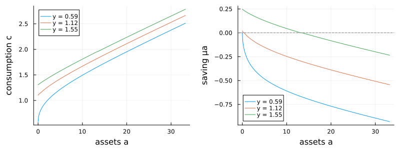

Consumption rises with both assets and income (left). Saving (right) tells the story of the borrowing constraint: at the limit $a = a_{\min}$ a low-income household would like to borrow but cannot, so its saving is pinned at zero and it consumes all of its income and interest. Because households are impatient relative to the interest rate ($\rho > r$), saving turns negative at high wealth — every income level has a finite target above which it runs its assets down — which is exactly what keeps the stationary wealth distribution from spreading without bound.

This page was generated using Literate.jl.