He–Krishnamurthy (2013): intermediary asset pricing

Households cannot hold the risky asset directly — they invest only through specialist intermediaries, and their equity stake in an intermediary is capped at a multiple $m$ of the intermediary's net worth. The single state $x$ is the specialists' wealth share. When $x$ falls the sector's risk-bearing capacity shrinks, the constraint binds, and the price of risk rises. The unknown is the specialists' wealth–consumption ratio $p_S$; goods-market clearing ties the aggregate price–consumption ratio $p$ to it.

The model

The parameters:

using EconPDEs, Plots

Base.@kwdef struct HeKrishnamurthy
  # See Table 2—Parameters and Targets
  m::Float64 = 4  # intermediation multiplier
  λ::Float64 = 0.6 # Debt/assets of intermediary sector
  g::Float64 = 0.02 # dividend growth
  σ::Float64 = 0.09 # dividend volatility
  ρ::Float64 = 0.04 # time discount rate
  γ::Float64 = 2.0 # risk aversion specialist
  l::Float64 = 1.84 # labor income ratio
end

Main.HeKrishnamurthy

We solve the model at its default parameters:

m = HeKrishnamurthy()

Main.HeKrishnamurthy(4.0, 0.6, 0.02, 0.09, 0.04, 2.0, 1.84)

The grid

We define the grid, a NamedTuple keyed by the state variable $x$, the specialists' wealth share. It runs over $(0, 1)$ — the endpoints are dropped — and is raised to the power $1.5$, which stretches points toward the lower boundary where specialists are poorly capitalized and the intermediation constraint bites.

xn = 100
stategrid =  (; x = range(0, 1, length = xn+2)[2:(end-1)].^1.5)

(x = [0.0009851853368415735, 0.002786524929624918, 0.00511917317484439, 0.007881482694732588, 0.01101470691806893, 0.014479208264002945, 0.018245887776131425, 0.022292199436999345, 0.02660000409472248, 0.031154295818195676  …  0.855224291261645, 0.8693600526303712, 0.8835728490716747, 0.8978622652870176, 0.9122278926230353, 0.9266693288961885, 0.9411861782238236, 0.9557780508613469, 0.970444563045229, 0.9851853368415734],)

The initial guess

We define the initial guess, a NamedTuple whose key is the single unknown function (pS, the specialists' wealth–consumption ratio), initialized flat at one. This name — and its finite differences, such as pSx_up — is what reappears inside the equation below.

guess = (; pS = ones(length(stategrid[:x])))

(pS = [1.0, 1.0, 1.0, 1.0, 1.0, 1.0, 1.0, 1.0, 1.0, 1.0  …  1.0, 1.0, 1.0, 1.0, 1.0, 1.0, 1.0, 1.0, 1.0, 1.0],)

The PDE equation

We now write the function encoding the equilibrium conditions. Following the package convention, it takes the current state (a grid point) and u — the local bundle holding the unknown and its finite-difference derivatives there (pS, pSx_up, pSx_down, pSxx) — and returns the time derivative pSt.

Goods-market clearing expresses the aggregate price–consumption ratio $p$ (and its derivatives) in terms of $p_S$. The state volatility $\sigma_x$ feeds back through prices, so the upwind direction is chosen from the drift $\mu_x$: forward pSx_up unless the drift turns negative, then backward pSx_down.

function (model::HeKrishnamurthy)(state::NamedTuple, u::NamedTuple)
  # `m` here is the intermediation multiplier (a model parameter), so the model instance is `model`.
  (; m, λ, g, σ, ρ, γ, l) = model
  (; pS, pSx_up, pSx_down, pSxx) = u
  (; x) = state
  iter = 0
  pSx = pSx_up
  @label start
  # market clearing for goods gives x / pS + (1 - x) * ρ = (1 + l) / p
  # This allows to obtain p (and its derivatives) in terms of pS (and its derivatives)
  p = (1 + l) / (x / pS + (1 - x) * ρ)
  px = - (1 + l) / (x / pS + (1 - x) * ρ)^2 * (1 / pS - ρ - x / pS^2 * pSx)
  pxx = - (1 + l) / (x / pS + (1 - x) * ρ)^2 * (- 1 / pS^2 * pSx - 1 / pS^2 * pSx - x / pS^2 * pSxx + 2 * x / pS^3 * pSx^2) + 2 * (1 + l) / (x / pS + (1 - x) * ρ)^3 * (1 / pS - ρ - x / pS^2 * pSx)^2

  αI = 1 / (1 - λ * (1 - x))
  if x * (1 + m) * αI < 1
    αI = 1 / (x * (1 + m))
  end
  # we have the usual feeback loop between asset prices and wealth
  # σx = x * (αI - 1) * (σ + σp)
  σx = x * (αI - 1) * σ / (1 -  x * (αI - 1) * px / p)
  σpS = pSx / pS * σx
  σp = px / p * σx
  σR = σ + σp
  κ = γ * (αI * σR - σpS)
  μx = x * (1 - x) * ((αI - (1 - αI * x) / (1-x)) * κ * σR - 1 / pS + ρ - (αI - (1 - αI * x) / (1 - x)) * σR^2 - l / ((1 - x) * p))
  if (iter == 0) && (μx < 0)
    iter += 1
    pSx = pSx_down
    @goto start
  end
  μpS = pSx / pS * μx + 0.5 * pSxx / pS * σx^2
  μp = px / p * μx + 0.5 * pxx / p * σx^2
  r = 1 / p + g + μp + σ * σp - κ * σR
  σCS = κ / γ
  μCS = (r - ρ) / γ + (1 + 1 / γ) / (2 * γ) * κ^2
  pSt = - (1 / pS + μCS + μpS + σCS * σpS - r - κ * (σCS + σpS))
  μR = r + κ * σR
  σI = αI * σR
  (; pSt), (; pS, p, r, κ, σp, μR, σR, αI, μx, σx, x, px, pxx, σI)
end

Solving the model

With the grid, guess, and equation in hand, pdesolve solves the stationary system:

result = pdesolve(m, stategrid, guess)

EconPDEResult
  solution:      pS (100)
  saved:         pS, p, r, κ, σp, μR, σR, αI, μx, σx, x, px, pxx, σI
  residual_norm: 1.94e-09
  converged:     true (tolerance 1.49e-08)

The solution

We saved the price of risk $\kappa$ on the grid. It tends to be elevated when specialists are poorly capitalized (low $x$) — exactly the region where the intermediation constraint binds and the sector can absorb little risk.

xs = stategrid[:x]
plot(xs, result.saved.κ; xlabel = "specialists' wealth share x", ylabel = "price of risk κ", legend = false)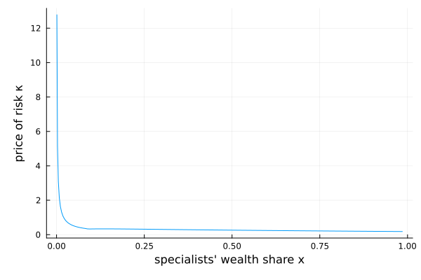

This page was generated using Literate.jl.