Di Tella (2017): uncertainty shocks and balance-sheet recessions

A two-state general-equilibrium model with a financial sector. Experts and households have recursive preferences and an agency friction (moral hazard) forces experts to bear idiosyncratic risk. There are two states: the experts' wealth share $x$ and a stochastic idiosyncratic risk state $\nu$ — the uncertainty shock. Three functions are solved jointly: transformed value/consumption objects $p_A, p_B$ for experts and households, and the capital price $p$, which is pinned down by an algebraic market-clearing constraint (is_algebraic) rather than by its own time derivative.

The model

The parameters:

using EconPDEs, Plots, Printf

Base.@kwdef struct DiTellaModel
  # Utility Function
  γ::Float64 = 5.0        # relative risk aversion
  ψ::Float64 = 2.0        # elasticity of intertemporal substitution
  ρ::Float64 = 0.0665     # rate of time preference (discount rate)
  τ::Float64 = 1.15       # transition rate between experts and households

  # Technology
  A::Float64 = 54.0       # investment adjustment-cost parameter calibrated to the paper targets
  δ::Float64 = 0.05       # depreciation rate in the investment technology
  B::Float64 = (0.20 - A * (0.02 + δ)^2) / (0.02 + δ)  # matches i(0.02) = 0.20
  σ::Float64 = 0.0125     # aggregate (fundamental) volatility of capital

  # MoralHazard
  ϕ::Float64 = 0.2        # moral-hazard idiosyncratic-risk retention parameter

  # Idiosyncratic
  νbar::Float64 = 0.25    # long-run mean of idiosyncratic risk state ν
  κν::Float64 = 1.38      # mean-reversion speed of ν (uncertainty process)
  σνbar::Float64 = -0.17  # volatility loading of the ν process
end

Main.DiTellaModel

The parameter values use the paper's reported calibration. The investment technology is $i(g)=A(g+\delta)^2+B(g+\delta)$ with $\delta=0.05$; the default $A$ and implied $B$ make the solved benchmark point near $x=0.10,\nu=0.25$ reproduce the paper's growth/investment targets, $g \simeq 0.02$ and $i \simeq 0.20$. We solve at these defaults:

m = DiTellaModel()

Main.DiTellaModel(5.0, 2.0, 0.0665, 1.15, 54.0, 0.05, -0.9228571428571434, 0.0125, 0.2, 0.25, 1.38, -0.17)

The grid

We define the grid, a NamedTuple keyed by the two state variables $x$ (the experts' wealth share) and $\nu$ (the idiosyncratic risk state), built by a helper. The $\nu$ range matches the horizontal range in Di Tella's Figure 1, and the grid explicitly includes the slices shown there: $x=0.05,0.10,0.20$ and $\nu=0.10,0.25,0.60$.

function initialize_stategrid(m::DiTellaModel; xn = 30, νn = 30)
  xs = sort(unique(vcat(collect(range(0.01, 0.99, length = xn)), [0.05, 0.10, 0.20])))
  νs = sort(unique(vcat(collect(range(0.01, 1.00, length = νn)), [0.10, 0.25, 0.60])))
  (; x = xs, ν = νs)
end

initialize_stategrid (generic function with 1 method)

The initial guess

We define the initial guess, a flat NamedTuple whose keys are the unknown functions (pA, pB, p), one starting value per grid point. The transformed objects pA and pB are convenient because 1 / pA and 1 / pB are the two agents' consumption rates, and Di Tella's relative investment opportunity measure is $Q = (p_A/p_B)^{1/(\psi-1)}$. These names — and their finite differences, e.g. pAx_up — are what reappear inside the equation below.

function initialize_guess(m::DiTellaModel, stategrid)
  xn = length(stategrid[:x])
  νn = length(stategrid[:ν])
  (; pA = ones(xn, νn), pB = ones(xn, νn), p = ones(xn, νn))
end

initialize_guess (generic function with 1 method)

We build the grid and the guess at the default calibration:

stategrid = initialize_stategrid(m)
guess = initialize_guess(m, stategrid)

(pA = [1.0 1.0 … 1.0 1.0; 1.0 1.0 … 1.0 1.0; … ; 1.0 1.0 … 1.0 1.0; 1.0 1.0 … 1.0 1.0], pB = [1.0 1.0 … 1.0 1.0; 1.0 1.0 … 1.0 1.0; … ; 1.0 1.0 … 1.0 1.0; 1.0 1.0 … 1.0 1.0], p = [1.0 1.0 … 1.0 1.0; 1.0 1.0 … 1.0 1.0; … ; 1.0 1.0 … 1.0 1.0; 1.0 1.0 … 1.0 1.0])

The PDE equation

We now write the function encoding the equilibrium conditions. Following the package convention, it takes the current state (a grid point) and u — the local bundle holding each unknown and its finite-difference derivatives there — and returns the time derivative of each unknown (pAt, pBt, pt).

With two states, both first derivatives and the cross derivative are upwinded — the first derivatives on the sign of their drifts, the cross term on the sign of the $x$–$\nu$ covariance.

function (m::DiTellaModel)(state::NamedTuple, u::NamedTuple)
  (; γ, ψ, ρ, τ, A, δ, B, σ, ϕ, νbar, κν, σνbar) = m
  (; x, ν) = state
  (; pA, pAx_up, pAx_down, pAν_up, pAν_down, pAxx, pAxν_up, pAxν_down, pAνν, pB, pBx_up, pBx_down, pBν_up, pBν_down, pBxx, pBxν_up, pBxν_down, pBνν, p, px_up, px_down, pν_up, pν_down, pxx, pxν_up, pxν_down, pνν) = u

  # drift and volatility of state variable ν
  q = (p - B) / (2 * A)
  g = q - δ
  i = A * q^2 + B * q
  μν = κν * (νbar - ν)
  σν = σνbar * sqrt(ν)
  pAν = (μν >= 0) ? pAν_up : pAν_down
  pBν = (μν >= 0) ? pBν_up : pBν_down
  pν = (μν >= 0) ? pν_up : pν_down

  pAx, pBx, px = pAx_up, pBx_up, px_up
  iter = 0
  @label start
  σX = x * (1 - x) * (1 - γ) / (γ * (ψ - 1)) * (pAν / pA - pBν / pB) * σν / (1 - x * (1 - x) * (1 - γ) / (γ * (ψ - 1)) * (pAx / pA - pBx / pB))
  σpA = pAx / pA * σX + pAν / pA * σν
  σpB = pBx / pB * σX + pBν / pB * σν
  σp = px / p * σX + pν / p * σν
  κ = (σp + σ - (1 - γ) / (γ * (ψ - 1)) * (x * σpA + (1 - x) * σpB)) / (1 / γ)
  # κidio is the price of idiosyncratic risk (distinct from the parameter κν, the mean-reversion speed of ν).
  κidio = γ * ϕ * ν / x
  σA = κ / γ + (1 - γ) / (γ * (ψ - 1)) * σpA
  νA = κidio / γ
  σB = κ / γ + (1 - γ) / (γ * (ψ - 1)) * σpB

  # Interest rate r
  μX = x * (1 - x) * ((σA * κ + νA * κidio - 1 / pA - τ) - (σB * κ -  1 / pB + τ * x / (1 - x)) - (σA - σB) * (σ + σp))

  # upwinding
  if (iter == 0) && (μX <= 0)
    iter += 1
    pAx, pBx, px = pAx_down, pBx_down, px_down
    @goto start
  end

  # upwind the cross derivative on the sign of its coefficient σX * σν (the x-ν covariance)
  pAxν = (σX * σν >= 0) ? pAxν_up : pAxν_down
  pBxν = (σX * σν >= 0) ? pBxν_up : pBxν_down
  pxν = (σX * σν >= 0) ? pxν_up : pxν_down

  μpA = pAx / pA * μX + pAν / pA * μν + 0.5 * pAxx / pA * σX^2 + 0.5 * pAνν / pA * σν^2 + pAxν / pA * σX * σν
  μpB = pBx / pB * μX + pBν / pB * μν + 0.5 * pBxx / pB * σX^2 + 0.5 * pBνν / pB * σν^2 + pBxν / pB * σX * σν
  μp = px / p * μX + pν / p * μν + 0.5 * pxx / p * σX^2 + 0.5 * pνν / p * σν^2 + pxν / p * σX * σν
  r = (1 - i) / p + g + μp + σ * σp - κ * (σ + σp) - γ / x * (ϕ * ν)^2

  # Market Pricing
  pAt = - pA * (1 / pA  + (ψ - 1) * τ / (1 - γ) * ((pA / pB)^((1 - γ) / (1 - ψ)) - 1) - ψ * ρ + (ψ - 1) * (r + κ * σA + κidio * νA) + μpA - (ψ - 1) * γ / 2 * (σA^2 + νA^2) + (2 - ψ - γ) / (2 * (ψ - 1)) * σpA^2 + (1 - γ) * σpA * σA)
  pBt = - pB * (1 / pB - ψ * ρ + (ψ - 1) * (r + κ * σB) + μpB - (ψ - 1) * γ / 2 * σB^2 + (2 - ψ - γ) / (2 * (ψ - 1)) * σpB^2 + (1 - γ) * σpB * σB)
  # algebraic constraint
  pt = - p * ((1 - i) / p - x / pA - (1 - x) / pB)
  Q = (pA / pB)^(1 / (ψ - 1))
  return (; pAt, pBt, pt), (; σx = σX, Q, r, κ, σp, growth = g, investment = i)
end

Solving the model

pdesolve solves the stationary system; p enters as an algebraic (constraint) variable rather than through its own time derivative:

result = pdesolve(m, stategrid, guess; is_algebraic = (; pA = false, pB = false, p = true))

EconPDEResult
  solution:      pA (33×33), pB (33×33), p (33×33)
  saved:         pA, pB, p, σx, Q, r, κ, σp, growth, investment
  residual_norm: 7.04e-10
  converged:     true (tolerance 1.49e-08)

The solution

We reproduce the three panels in Di Tella's Figure 1: the capital price $p$, the volatility of experts' wealth share $\sigma_x$, and relative investment opportunities $Q$. Each object is plotted both as a function of uncertainty $\nu$ at fixed balance sheets and as a function of experts' wealth share $x$ at fixed uncertainty. The key Di Tella mechanism is that an uncertainty shock raises the idiosyncratic risk experts must retain. When experts' balance sheets are weak (low $x$), their risk-bearing capacity is low, so the same increase in $\nu$ produces a larger fall in the capital price and a larger balance-sheet response.

xs = stategrid[:x]
νs = stategrid[:ν]
p = result.solution.p
σx = result.saved.σx
Q = result.saved.Q
line_styles = [:solid, :dot, :dash]
x_slices = [0.05, 0.10, 0.20]
ν_slices = [0.10, 0.25, 0.60]

pν = plot(; xlabel = "risk state ν", ylabel = "capital price p",
          xlims = (0, 1), ylims = (5.6, 7.2), legend = :bottomleft)
σxν = plot(; xlabel = "risk state ν", ylabel = "volatility σx",
           xlims = (0, 1), ylims = (0, 0.01), legend = false)
Qν = plot(; xlabel = "risk state ν", ylabel = "relative opportunities Q",
          xlims = (0, 1), ylims = (1.0, 2.7), legend = false)
for (x_slice, line_style) in zip(x_slices, line_styles)
  x_index = findfirst(==(x_slice), xs)
  plot!(pν, νs, p[x_index, :]; label = @sprintf("x = %.2f", x_slice),
        color = :black, linestyle = line_style)
  plot!(σxν, νs, σx[x_index, :]; color = :black, linestyle = line_style)
  plot!(Qν, νs, Q[x_index, :]; color = :black, linestyle = line_style)
end
px = plot(; xlabel = "wealth share x", ylabel = "capital price p",
          xlims = (0, 1), ylims = (5.6, 7.2), legend = :bottomright)
σxx = plot(; xlabel = "wealth share x", ylabel = "volatility σx",
           xlims = (0, 1), ylims = (0, 0.01), legend = false)
Qx = plot(; xlabel = "wealth share x", ylabel = "relative opportunities Q",
          xlims = (0, 1), ylims = (1.0, 2.7), legend = false)
for (ν_slice, line_style) in zip(ν_slices, line_styles)
  ν_index = findfirst(==(ν_slice), νs)
  plot!(px, xs, p[:, ν_index]; label = @sprintf("ν = %.2f", ν_slice),
        color = :black, linestyle = line_style)
  plot!(σxx, xs, σx[:, ν_index]; color = :black, linestyle = line_style)
  plot!(Qx, xs, Q[:, ν_index]; color = :black, linestyle = line_style)
end
plot(pν, σxν, Qν, px, σxx, Qx; layout = (2, 3), size = (940, 560),
     left_margin = 8Plots.mm, bottom_margin = 8Plots.mm, right_margin = 4Plots.mm)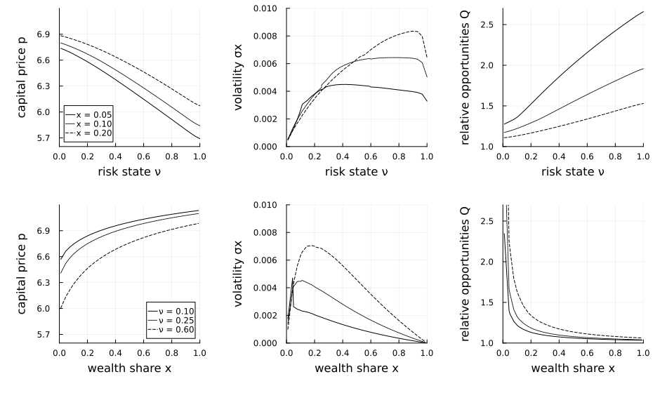

This page was generated using Literate.jl.