Achdou–Han–Lasry–Lions–Moll: portfolio choice with two assets
This extends the Achdou–Han–Lasry–Lions–Moll consumption–saving problem to a portfolio choice between a riskless asset (return $r$) and a risky asset (return $\mu_R$, volatility $\sigma_R$). A household with total wealth $a$ chooses consumption $c$ and how much of its wealth $k$ to hold in the risky asset, subject to no short-selling and no leverage ($0 \le k \le a - a_{\min}$). Labor income $y$ follows the same mean-reverting diffusion. Wealth evolves as $da = \bigl(y + r a + (\mu_R - r) k - c\bigr)dt + \sigma_R k\, dW$ and the value function $v(y, a)$ solves
\[\rho\, v = \max_{c,\,k}\; \frac{c^{1-\gamma}}{1-\gamma} + \partial_a v\,\bigl(y + r a + (\mu_R - r) k - c\bigr) + \tfrac12 \sigma_R^2 k^2\, \partial_{aa} v + \partial_y v\,\kappa_y(\bar y - y) + \tfrac12 \sigma_y^2\, \partial_{yy} v.\]
The first-order conditions are $c = (\partial_a v)^{-1/\gamma}$ for consumption and the Merton rule $k = -\tfrac{\mu_R - r}{\sigma_R^2}\,\partial_a v / \partial_{aa} v$ for the risky holding, clamped to $[0, a - a_{\min}]$. Those formulas are used only when the local value derivatives make the Hamiltonian concave in the relevant control; otherwise the bounded Hamiltonian is maximized directly.
The model
The parameters live in a struct:
using EconPDEs, Distributions, Plots

Base.@kwdef struct AchdouHanLasryLionsMollModel_RiskyAsset
    κy::Float64 = 0.1        # mean-reversion speed of labor income
    ybar::Float64 = 1.0      # long-run mean of labor income
    σy::Float64 = 0.07       # volatility of labor income

    r::Float64 = 0.03        # risk-free rate
    μR::Float64 = 0.04       # expected return on the risky asset
    σR::Float64 = 0.1        # volatility of the risky asset

    ρ::Float64 = 0.05        # discount rate
    γ::Float64 = 2.0         # relative risk aversion

    amin::Float64 = 0.0      # borrowing limit (minimum wealth)
    amax::Float64 = 300.0    # maximum wealth (grid upper bound)
end

function _merton_consumption_rate(m::AchdouHanLasryLionsMollModel_RiskyAsset)
    prem = m.μR - m.r
    return (m.ρ - m.r) / m.γ + m.r - (1 - m.γ) * prem^2 / (2 * m.γ^2 * m.σR^2)
end
_merton_consumption_rate (generic function with 1 method)We solve the model at its default parameters:
m = AchdouHanLasryLionsMollModel_RiskyAsset()Main.AchdouHanLasryLionsMollModel_RiskyAsset(0.1, 1.0, 0.07, 0.03, 0.04, 0.1, 0.05, 2.0, 0.0, 300.0)The grid
We define the grid, a NamedTuple keyed by income $y$ and wealth $a$. Income spans the bulk of its ergodic (Gamma) distribution; wealth uses a curved grid, finer near the borrowing constraint, where the constraint and the risky-share tilt create most of the curvature.
distribution = Gamma(2 * m.κy * m.ybar / m.σy^2, m.σy^2 / (2 * m.κy))
ys = collect(range(quantile(distribution, 0.001), quantile(distribution, 0.999), length = 5))
as = m.amin .+ (m.amax - m.amin) .* collect(range(0.0, 1.0, length = 150)).^2
stategrid = (; y = ys, a = as)
(y = [0.5850212023872049, 0.8273003253744176, 1.06957944836163, 1.3118585713488429, 1.5541376943360554], a = [0.0, 0.013512904824107023, 0.05405161929642809, 0.12161614341696318, 0.21620647718571237, 0.3378226206026756, 0.48646457366785273, 0.6621323363812441, 0.8648259087428495, 1.094545290752669 … 264.85293455249763, 268.6500608080717, 272.474212873294, 276.32539074816447, 280.20359443268325, 284.10882392685016, 288.0410792306653, 292.00036034412864, 295.9866672672402, 300.0])The initial guess
We define the initial guess, a NamedTuple keyed by the unknown $v$ — here the Merton-tail value of consuming out of financial plus human wealth $a + y/r$. These names (and the finite differences of $v$, such as va_up) are what reappear in the equation below.
cshare = _merton_consumption_rate(m)
guess = (; v = [cshare^(-m.γ) * (a + y / m.r)^(1 - m.γ) / (1 - m.γ) for y in stategrid[:y], a in stategrid[:a]])
(v = [-30.137119684802666 -30.116250798561996 … -1.8628166499131185 -1.839417318148372; -21.31131035940428 -21.300872674697942 … -1.8163217268933123 -1.794068911170538; … ; -13.439599648582886 -13.435447861213813 … -1.729963757384709 -1.7097649150733216; -11.344460699167618 -11.34150233887124 … -1.6897927167189477 -1.6705158209137319],)The PDE equation
We now write the function encoding the HJB equation. Following the package convention, it takes the current state (a grid point) and u (each unknown together with its finite-difference derivatives there) and returns the time derivative of each unknown.
As in the one-asset model, income is upwinded on $\mu_y$ and the endogenous asset drift picks the forward/backward derivative that keeps its sign consistent. At each candidate we use the closed-form FOCs when they are well posed and otherwise maximize the bounded local Hamiltonian. The boundary branches impose the borrowing constraint at $a_{\min}$ and a homothetic tail at $a_{\max}$. We save consumption $c$, the risky holding $k$, and the saving rate $\mu_a$ on the grid.
function (m::AchdouHanLasryLionsMollModel_RiskyAsset)(state::NamedTuple, u::NamedTuple)
    (; κy, σy, ybar, r, μR, σR, ρ, γ, amin, amax) = m
    (; y, a) = state
    (; v, vy_up, vy_down, va_up, va_down, vyy, vaa) = u
    μy = κy * (ybar - y)
    cash = y + r * a
    prem = μR - r
    kmax = max(a - amin, 0.0)
    # Newton can try negative marginal values, so cap implied consumption instead of flooring derivatives.
    cmax = max(100.0 * (y + r * max(a, 0.0)), sqrt(eps()))
    cmin = sqrt(eps())

    if (a ≈ amax)
        va_tail = (isfinite(va_down) && va_down > 0.0) ? va_down : va_up
        vaa = - m.γ * va_tail / a
    end

    # upwinding for income direction (easy because exogenous income drift)
    vy = (μy >= 0) ? vy_up : vy_down

    function policy_candidate(va_candidate)
        c_candidate = va_candidate > 0.0 ? clamp(va_candidate^(-1 / γ), cmin, cmax) : cmax
        # First compare the two portfolio constraints, then add the Merton interior point if it
        # is well-defined. This keeps Newton's off-path trial values finite without hiding the FOC.
        # Portfolio Hamiltonian at the upper constraint.
        H_kmax = prem * va_candidate * kmax + 0.5 * vaa * σR^2 * kmax^2
        k_candidate = H_kmax > 0.0 ? kmax : 0.0
        if va_candidate > 0.0 && vaa < 0.0
            k_merton = clamp(-prem * va_candidate / (σR^2 * vaa), 0.0, kmax)
            # Compare the interior Merton point with the best constraint found above.
            H_merton = prem * va_candidate * k_merton + 0.5 * vaa * σR^2 * k_merton^2
            H_candidate = prem * va_candidate * k_candidate + 0.5 * vaa * σR^2 * k_candidate^2
            k_candidate = H_merton >= H_candidate ? k_merton : k_candidate
        end
        μa_candidate = cash + prem * k_candidate - c_candidate
        return c_candidate, k_candidate, μa_candidate
    end

    # upwinding for asset direction (harder because endogeneous asset drift)
    c_up, k_up, μa_up = policy_candidate(va_up)
    if μa_up >= 0.0
        va = va_up
        c = c_up
        k = k_up
        μa = μa_up
    else
        c_down, k_down, μa_down = policy_candidate(va_down)
        if (μa_down <= 0.0) && (a > amin)
            va = va_down
            c = c_down
            k = k_down
            μa = μa_down
        else
            # If the two candidates straddle zero OR drift is negative at minimum asset threshold
            # (i.e. borrowing constraint), then, we must have drift μa = 0. When the zero-drift
            # Hamiltonian is concave we solve its FOC by bisection; otherwise we compare endpoints.
            k_hi = kmax
            if prem < 0.0
                k_hi = min(k_hi, max((cash - cmin) / (-prem), 0.0))
            end

            if k_hi == 0.0 || !(isfinite(cash) && isfinite(prem) && isfinite(vaa) && isfinite(σR))
                k = 0.0
            elseif vaa < 0.0 && σR > 0.0
                dh0 = prem * max(cash, cmin)^(-γ)
                dh1 = prem * max(cash + prem * k_hi, cmin)^(-γ) + vaa * σR^2 * k_hi
                if isfinite(dh0) && isfinite(dh1)
                    if dh0 <= 0.0
                        k = 0.0
                    elseif dh1 >= 0.0
                        k = k_hi
                    else
                        lo, hi = 0.0, k_hi
                        for _ in 1:40
                            mid = (lo + hi) / 2.0
                            dh = prem * max(cash + prem * mid, cmin)^(-γ) + vaa * σR^2 * mid
                            if dh > 0.0
                                lo = mid
                            else
                                hi = mid
                            end
                        end
                        k = (lo + hi) / 2.0
                    end
                else
                    k = 0.0
                end
            else
                c0 = max(cash, cmin)
                c1 = max(cash + prem * k_hi, cmin)
                h0 = c0^(1 - γ) / (1 - γ)
                h1 = c1^(1 - γ) / (1 - γ) + 0.5 * vaa * σR^2 * k_hi^2
                k = h1 > h0 ? k_hi : 0.0
            end
            c = max(cash + prem * k, cmin)
            va = c^(-γ)
            μa = 0.0
        end
    end
    σa = k * σR
    vt = - (c^(1 - γ) / (1 - γ) + va * μa + 0.5 * vaa * σa^2 + vy * μy + 0.5 * vyy * σy^2 - ρ * v)
    return (; vt), (; v, c, k, va, vaa, vy, y, a, μa)
end
Solving the model
With the grid, guess, and equation in hand, pdesolve solves the stationary system. The upper derivative boundary is the homothetic Merton tail; this matters because the risky asset gives wealth a nonzero diffusion near the top of the grid.
bc = (; va = ((stategrid.y .+ m.r * m.amin).^(-m.γ),
              fill(cshare^(-m.γ) * m.amax^(-m.γ), length(stategrid.y))))

result = pdesolve(m, stategrid, guess; bc)
EconPDEResult
solution: v (5×150)
saved: v, c, k, va, vaa, vy, y, a, μa
residual_norm: 6.55e-11
converged: true (tolerance 1.49e-08)The solution
We plot the two policies against wealth for three income levels (low, median, high).
as = stategrid[:a]
ys = stategrid[:y]
idx = 1:div(length(as), 3)          # left third of the wealth grid, where the curvature is
iys = round.(Int, range(1, length(ys), length = 3))

p1 = plot(xlabel = "wealth a", ylabel = "consumption c")
for iy in iys
    plot!(p1, as[idx], result.saved.c[iy, idx], label = "y = $(round(ys[iy], digits = 2))")
end
p2 = plot(xlabel = "wealth a", ylabel = "saving μa")
for iy in iys
    plot!(p2, as[idx], result.saved.μa[iy, idx], label = "y = $(round(ys[iy], digits = 2))")
end
hline!(p2, [0.0]; color = :gray, linestyle = :dash, label = "")
plot(p1, p2; layout = (1, 2), size = (800, 300))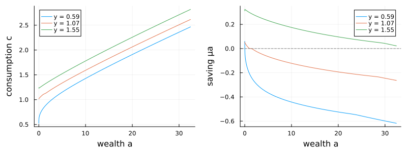
Consumption rises with both wealth and income (left); the saving rate (right) is highest for the wealth-poor and turns negative as households approach their target wealth. On the portfolio side (not shown), away from the constraint the household holds the Merton fraction $(\mu_R - r)/(\gamma\sigma_R^2)$ of wealth in the risky asset, and tilts toward the safe asset near the constraint, where it cannot lever and labor-income risk crowds out financial risk-taking.
This page was generated using Literate.jl.