Bansal–Yaron (2004): long-run risk (two states)

The long-run-risk model has two state variables, so it exercises the package's 2D machinery — a matrix of unknowns and a sparse Jacobian on a genuine grid. Consumption growth has a small, persistent expected-growth component $\mu$ and a stochastic variance $v$:

\[d\mu = \kappa_\mu(\bar\mu - \mu)\,dt + \nu_\mu\sqrt{v}\,dW_\mu, \qquad dv = \kappa_v(\bar v - v)\,dt + \nu_v\sqrt{v}\,dW_v.\]

With Epstein–Zin preferences the unknown is the wealth–consumption ratio $p(\mu, v)$, which solves a nonlinear elliptic PDE. The gradient-nonlinear risk terms $\sigma_\mu^2 p_\mu^2/p$ and $\sigma_v^2 p_v^2/p$ come from the market prices of long-run-risk and variance risk.

The model

The parameters live in a struct:

using EconPDEs, Distributions, Plots

Base.@kwdef struct BansalYaronModel
    μbar::Float64 = 0.018    # long-run mean of expected consumption growth
    vbar::Float64 = 0.00073  # long-run mean of consumption variance
    κμ::Float64 = 0.252      # mean-reversion speed of expected growth
    νμ::Float64 = 0.528      # volatility of expected growth
    κv::Float64 = 0.156      # mean-reversion speed of variance
    νv::Float64 = 0.00354    # volatility of variance (vol of vol)
    ρ::Float64 = 0.024       # discount rate
    γ::Float64 = 7.5         # relative risk aversion
    ψ::Float64 = 1.5         # elasticity of intertemporal substitution
end

Main.BansalYaronModel

We solve the model at its default parameters:

m = BansalYaronModel()

Main.BansalYaronModel(0.018, 0.00073, 0.252, 0.528, 0.156, 0.00354, 0.024, 7.5, 1.5)

The grid

We define the grid, a NamedTuple with two keys (μ and v), one per state variable. The grid spans the ergodic ranges of $\mu$ (Normal) and $v$ (Gamma). The $\sqrt v$ diffusion vanishes at $v = 0$, a degenerate boundary where no condition is imposed.

μn, vn = 30, 30
μdistribution = Normal(m.μbar, sqrt(m.νμ^2 * m.vbar / (2 * m.κμ)))
μs = range(quantile(μdistribution, 0.01), quantile(μdistribution, 0.99), length = μn)
νdistribution = Gamma(2 * m.κv * m.vbar / m.νv^2, m.νv^2 / (2 * m.κv))
vs = range(quantile(νdistribution, 0.0), quantile(νdistribution, 0.99), length = vn)
stategrid = (; μ = μs, v = vs)

(μ = -0.02874710735595003:0.0032239384383413814:0.06474710735595003, v = 0.0:4.090285065742189e-5:0.0011861826690652349)

The initial guess

We define the initial guess, a NamedTuple whose key is the unknown function (p, the wealth–consumption ratio), a matrix over the $(\mu, v)$ grid. These names (and the finite differences of $p$, such as pμ_up and pμμ) are what reappear in the equation below.

guess = (; p = ones(μn, vn))

(p = [1.0 1.0 … 1.0 1.0; 1.0 1.0 … 1.0 1.0; … ; 1.0 1.0 … 1.0 1.0; 1.0 1.0 … 1.0 1.0],)

The PDE equation

We now write the function encoding the HJB equation. Following the package convention, it takes the current state (a grid point) and u (each unknown together with its finite-difference derivatives there) and returns the time derivative of each unknown.

function (m::BansalYaronModel)(state::NamedTuple, u::NamedTuple)
    (; μbar, vbar, κμ, νμ, κv, νv, ρ, γ, ψ) = m
    (; μ, v) = state
    (; p, pμ_up, pμ_down, pv_up, pv_down, pμμ, pvv) = u

    # drifts and volatilities of consumption, μ and v
    μc = μ
    σc = sqrt(v)
    μμ = κμ * (μbar - μ)
    σμ = νμ * sqrt(v)
    μv = κv * (vbar - v)
    σv = νv * sqrt(v)

    # upwind each first derivative on the sign of its drift
    pμ = (μμ >= 0) ? pμ_up : pμ_down
    pv = (μv >= 0) ? pv_up : pv_down

    σp_Zμ = pμ / p * σμ
    σp_Zv = pv / p * σv
    σp2 = σp_Zμ^2 + σp_Zv^2
    μp = pμ / p * μμ + pv / p * μv + 0.5 * pμμ / p * σμ^2 + 0.5 * pvv / p * σv^2

    # market prices of risk
    κ_Zc = γ * σc
    κ_Zμ = -(1 - γ * ψ) / (ψ - 1) * σp_Zμ
    κ_Zv = -(1 - γ * ψ) / (ψ - 1) * σp_Zv

    r = ρ + μc / ψ - (1 + 1 / ψ) / 2 * γ * σc^2 - (γ * ψ - 1) / (2 * (ψ - 1)) * σp2
    pt = -p * (1 / p + μc + μp - r - κ_Zc * σc - κ_Zμ * σp_Zμ - κ_Zv * σp_Zv)
    return (; pt)
end

Solving the model

With the grid, guess, and equation in hand, pdesolve solves the stationary system:

result = pdesolve(m, stategrid, guess)

EconPDEResult
  solution:      p (30×30)
  residual_norm: 1.40e-09
  converged:     true (tolerance 1.49e-08)

The solution

The wealth–consumption ratio increases in expected growth $\mu$ and falls with variance $v$: investors pay more for the claim when future growth is high, and less when the economy is riskier. Because $p$ is defined over the $(\mu, v)$ plane, we show the full state-space pattern as a three-dimensional graph.

p = result.solution.p
surface(vs, μs, p; xlabel = "variance v", ylabel = "growth μ", zlabel = "p", colorbar = false, size = (720, 460), left_margin = 8Plots.mm, bottom_margin = 8Plots.mm, right_margin = 6Plots.mm)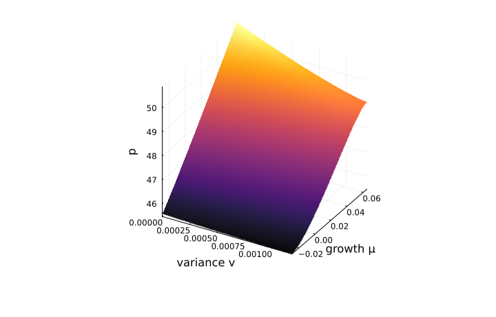

This page was generated using Literate.jl.